← return to practice.dsc80.com
Instructor(s): Suraj Rampure
This exam was administered in-person. The exam was closed-notes, except students were allowed to bring 2 two-sided cheat sheets. No calculators were allowed. Students had 180 minutes to take this exam.
The DataFrame sat contains one row for
most combinations of "Year" and
"State", where "Year" ranges between
2005 and 2015 and "State" is one
of the 50 states (not including the District of Columbia).
The other columns are as follows:
"# Students" contains the number of students who
took the SAT in that state in that year.
"Math" contains the mean math section score among
all students who took the SAT in that state in that year. This ranges
from 200 to 800.
"Verbal" contains the mean verbal section score
among all students who took the SAT in that state in that year. This
ranges from 200 to 800. (This is now known as the “Critical Reading”
section.)
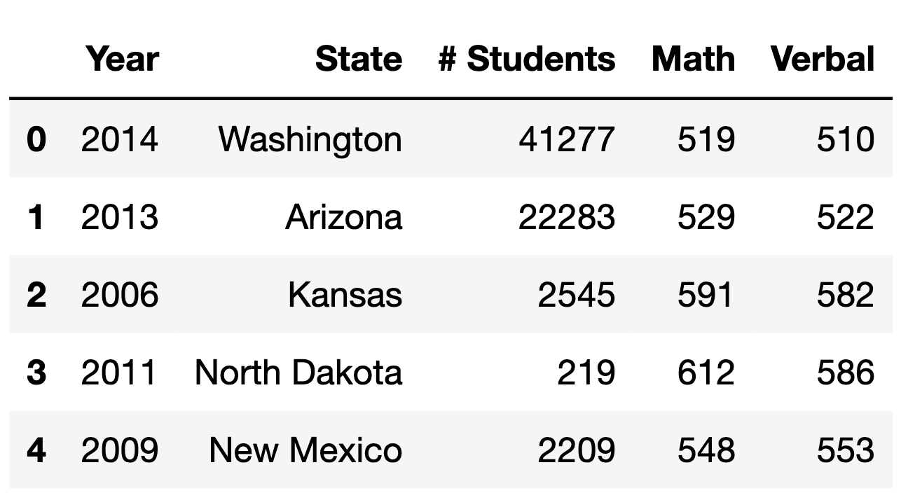
The first few rows of sat are shown below (though
sat has many more rows than are pictured here).
For instance, the first row of sat tells us that 41227
students took the SAT in Washington in 2014, and among those students,
the mean math score was 519 and the mean verbal score was 510.
Assume:
sat does not contain any duplicate rows — that is,
there is only one row for every unique combination of
"Year" and "State" that is in
sat.
sat does not contain any null values.
We have already run all of the necessary imports.
Which of the following expressions evaluate to the name of the state, as a string, with the highest mean math section score in 2007? Select all that apply.
Note: Assume that the highest mean math section score in 2007 was unique to only one state.
Option 1:
(sat.loc[(sat["Math"] == sat["Math"].max()) &
       (sat["Year"] == 2007), "State"]
.iloc[0])
Option 2:
sat.loc[sat["Year"] == 2007].set_index("State")["Math"].idxmax()Option 3:
sat.groupby("Year")["State"].max().loc[2007]Option 4:
(sat.loc[sat["Math"] == sat.loc[sat["Year"] == 2007, "Math"].max()]
   .iloc[0]
   .loc["State"])
Option 5:
(sat.groupby("Year").apply(
    lambda sat: sat[sat["Math"] == sat["Math"].max()]
).reset_index(drop=True)
.groupby("Year")["State"].max()
.loc[2007])
Option 6:
sat.loc[sat['Year'] == 2007].loc[sat['Math'] == sat['Math'].max()]Option 1
Option 2
Option 3
Option 4
Option 5
Option 6
None of the above
Answer: Option 2 and Option 5
Option 1:
(sat.loc[(sat["Math"] == sat["Math"].max()) & (sat["Year"] == 2007), "State"].iloc[0])
This expression looks for entries where the math score equals the
overall max "Math" score in the dataset and the year is
2007. However, this approach has a limitation: it assumes that the
highest math score in the entire dataset occurred in 2007.
Option 2:
sat.loc[sat["Year"] == 2007].set_index("State")["Math"].idxmax()
After boolean indexing for entries made in 2007, it correctly returns
the state name with the max "Math" score.
Option 3: sat.groupby("Year")["State"].max().loc[2007]
This finds the maximum state name alphabet-wise, not the state with the
highest math score.
Option 4:
(sat.loc[sat["Math"] == sat.loc[sat["Year"] == 2007, "Math"].max()].iloc[0].loc["State"])
This expression looks to match any recorded score that is equal to the
max score in 2007, possibly returning a value outside of 2007.
Option 5:
(sat.groupby("Year").apply(lambda sat: sat[sat["Math"] == sat["Math"].max()]).reset_index(drop=True).groupby("Year")["State"].max().loc[2007])
Option 5 works by isolating rows with the highest score per year, and
then among these, it finds the state for the year 2007.
Option 6:
sat.loc[sat['Year'] == 2007].loc[sat['Math'] == sat['Math'].max()]
Similar to Option 4, this expression finds the maximum math score across
all years and then tries to match it to the year 2007, which may not be
correct.
The average score on this problem was 71%.
Note that this problem is no longer in scope.
In the box, write a one-line expression that evaluates to a DataFrame that is equivalent to the following relation:
\Pi_{\text{Year, State, Verbal}} \left(\sigma_{\text{Year } \geq \: 2014 \text{ and Math } \leq \: 600} \left( \text{sat} \right) \right)
Answer:
sat.loc[(sat['Year'] >= 2014) & (sat['Math'] <= 600), ['Year', 'State', 'Verbal']]
The average score on this problem was 85%.
The following two lines define two DataFrames, val1 and
val2.
val1 = sat.groupby(["Year", "State"]).max().reset_index()
val2 = sat.groupby(["Year", "State", "# Students"]).min().reset_index()
Are val1 and val2 identical? That is, do
they contain the same rows and columns, all in the same order?
Yes
No
Answer: Yes
No pair of "Year" and "State" will be
appear twice in the DataFrame because each combination of
"Year" and "State" are unqiue. Therefore, when
grouping by these columns, each group only contains one unique row - the
row itself. Thus, using the maximum operation on these groups simply
retrieves the original rows.
Likewise, since every combination of "Year",
"State", and "# Students" is also unique, the
minimum operation, when applied after grouping, yields the same result:
the original row for each group.
Recall that .groupby function in Pandas automatically
sorts data based on the chosen grouping keys. As a result, the
val1 and val2 DataFrames, created using these
groupings, contain the same rows and columns, displayed in the same
order.
The average score on this problem was 67%.
The data description stated that there is one row in sat
for most combinations of "Year" (between 2005
and 2015, inclusive) and "State". This means
that for most states, there are 11 rows in sat — one for
each year between 2005 and 2015, inclusive.
It turns out that there are 11 rows in sat for all 50
states, except for one state. Fill in the blanks below so that
missing_years evaluates to an array,
sorted in any order, containing the years for which that one state does
not appear in `sat.
state_only = sat.groupby("State").filter(___(a)___)

merged = sat["Year"].value_counts().to_frame().merge(
    state_only, ___(b)___
)

missing_years = ___(c)___.to_numpy()
What goes in the blanks?
Answer:
lambda df: df.shape[0] < 11left_index=True, right_on='Year', how='left'
(how='outer' also works)merged[merged['# Students'].isna()]['Year']The initial step (in the state_only variable) involves
identifying the state that has fewer than 11 records in the dataset.
This is achieved by the lambda function
lambda df: df.shape[0] < 11, leaving us with records
from only the state that has missing data for certain years.
The average score on this problem was 72%.
Next, applying .value_counts() to
sat["Year"] produces a Series that enumerates the total
occurrences of each year from 2005 to 2015. Converting this Series to a
DataFrame with .to_frame(), we then merge it with the
state_only DataFrame. This merging results in a DataFrame
(merged) where the years lacking corresponding entries in
state_only are marked as NaN.
The average score on this problem was 52%.
Finally, the expression
merged[merged['# Students'].isna()]['Year'] in
missing_years identifies the specific years that are absent
for the one state in the sat dataset. This is determined by selecting
years in the merged DataFrame where the "# Students" column
has NaN values, indicating missing data for those years.
The average score on this problem was 71%.
In the previous subpart, we established that most states have 11 rows
in sat — one for each year between 2005 and 2015, inclusive
— while there is one state that has fewer than 11 rows, because there
are some years for which that state’s SAT information is not known.
Suppose we’re given a version of sat called
sat_complete that has all of the same information as
sat, but that also has rows for combinations of states and
years in which SAT information is not known. While there are no null
values in the "Year" or "State" columns of
sat_complete, there are null values in the
"# Students", "Math", and
"Verbal" columns of sat_complete. An example
of what sat_complete may look like is given below.
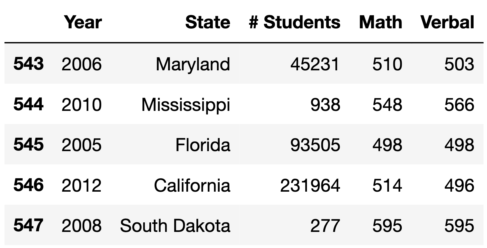
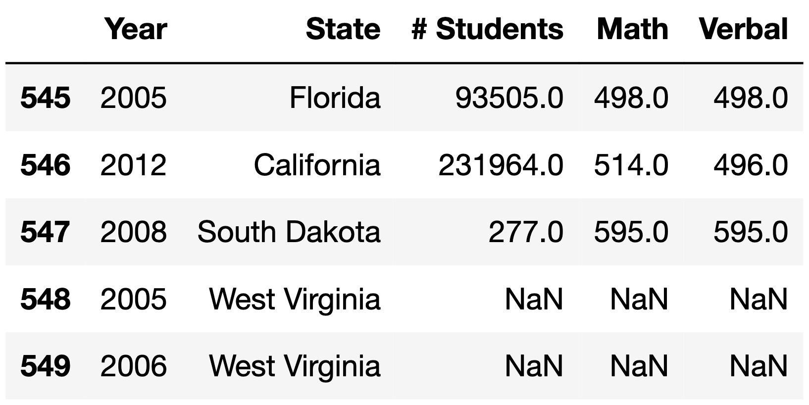
Note that in the above example, sat simply wouldn’t
have rows for West Virginia in 2005 and 2006, meaning it would have 2
fewer rows than the corresponding sat_complete.
Given just the information in sat_complete — that is,
without including any information learned in part (d) — what is the most
likely missingness mechanism of the "# Students" column in
sat_complete?
Not missing at random
Missing at random
Missing completely at random
Answer: Not missing at random
The fact that there are null values specifically in the cases where
SAT data is not available suggests that the missingness of the
"# Students" column is systematic. It’s not occurring
randomly across the dataset, but rather in specific instances where SAT
data wasn’t recorded or available.
This could mean that the absence of student numbers is linked to specific reasons why the data was not recorded or collected, such as certain states not participating in SAT testing in specific years, or administrative decisions that led to non-recording of data.
The nature of this missingness suggests that it’s not random or
solely dependent on observed data in other columns, but rather it’s
related to the inherent nature of the "# Students" data
itself.
The average score on this problem was 54%.
Given just the information in sat_complete — that is,
without including any information learned in part (d) — what is the most
likely missingness mechanism of the "Math" column in
sat_complete?
Not missing at random
Missing at random
Missing completely at random
Answer: Missing at random
If a state has reported the number of students taking the SAT, it
implies that data collection and reporting were carried out. The
administrative decision to report SAT scores (including
"Math" scores) may be reflected in the
"# Students" column. Conversely, if the
"# Students" column is empty or null for a certain state
and year, it might indicate an administrative decision not to
participate or report data for that period. This decision impacts the
availability of "Math" scores.
In this context, the missing values in "Math" scores are
linked to observable conditions or patterns in the dataset (like
specific years, states, or availability of other related data).
The average score on this problem was 75%.
Suppose we perform a permutation test to assess whether the missingness of column Y depends on column X.
Suppose we observe a statistically significant result (that is, the p-value of our test is less than 0.05). True or False: It is still possible for column Y to be not missing at random.
True
False
Answer: True
The observation of a statistically significant result (a p-value less than 0.05) in a permutation test suggests there is some association or dependency between the missingness in Y and the values in X. However, this result does not exclude the possibility that the missingness in Y is also influenced by factors not captured in column X, or by the values in Y itself.
The average score on this problem was 71%.
Suppose we do not observe a statistically significant result (that is, the p-value of our test is greater than 0.05). True or False: It is still possible for column Y to be missing at random dependent on column X.
True
False
Answer: True
Not observing a statistically significant result (a p-value greater than 0.05) in a permutation test means that the test did not find strong evidence of a dependency between X and the missingness in Y. However, this does not definitively prove that such a dependency does not exist. In statistical testing, a lack of significant findings is not the same as evidence of no effect or no association.
The average score on this problem was 78%.
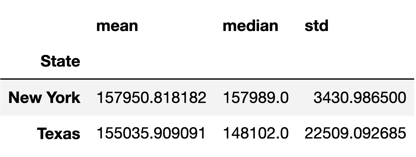
The following DataFrame contains the mean, median, and standard deviation of the number of students per year who took the SAT in New York and Texas between 2005 and 2015.
Which of the following expressions creates the above DataFrame correctly and in the most efficient possible way (in terms of time and space complexity)?
Note: The only difference between the options is the positioning
of "# Students".
Option 1:
(sat.loc[sat["State"].isin(["New York", "Texas"])]
["# Students"].groupby("State").agg(["mean", "median", "std"]))
Option 2:
(sat.loc[sat["State"].isin(["New York", "Texas"])]
.groupby("State")["# Students"].agg(["mean", "median", "std"]))
Option 3:
(sat.loc[sat["State"].isin(["New York", "Texas"])]
.groupby("State").agg(["mean", "median", "std"])["# Students"])
Option 1
Option 2
Option 3
Multiple options are equally correct and efficient
Answer: Option 2
"# Students" column before grouping by
"State", which is not possible."State", and
then performs aggregation only on the "# Students" column,
making it efficient."# Students" column, which is correct but less
efficient because it computes aggregations for potentially many columns
(like "Math") that are not needed.
The average score on this problem was 75%.
Suppose we want to run a statistical test to assess whether the distributions of the number of students between 2005 and 2015 in New York and Texas are significantly different.
What type of test is being proposed above?
Hypothesis test
Permutation test
Answer: Permutation test
Here, we’re comparing whether two sample distributions –
specifically, (1) the distribution of the number of students per year
from 2005-2015 for New York and (2) the distribution of the number of
students per year from 2005-2015 for Texas – are significantly
different. This is precisely what a permutation test is used for. For
the purposes of this test, we have 22 relevant rows of data – 11 for New
York and 11 for Texas – and 2 columns, "State" and
"# Students".
The average score on this problem was 90%.
Given the information in the above DataFrame, which test statistic is most likely to yield a significant difference?
\text{mean number of students in Texas } - \text{ mean number of students in New York}
\big|\text{mean number of students in Texas } - \text{ mean number of students in New York}\big|
\big|\text{median number of students in Texas } - \text{ median number of students in New York}\big|
The Kolmogorov-Smirnov statistic
Answer: The Kolmogorov-Smirnov statistic
Here, the means and medians of the two samples are similar, so their observed difference in means and observed difference in medians are both small. This means that a permutation test using either one of those as a test statistic will likely fail to yield a significant difference. However, the standard deviations of both distributions are quite different, which means the shapes of the distributions are quite different. The Kolmogorov-Smirnov statistic measures the distance between two distributions by considering their entire shape, and since these distributions have very different shapes, they will likely have a larger Kolmogorov-Smirnov statistic than expected under the null.
The average score on this problem was 78%.
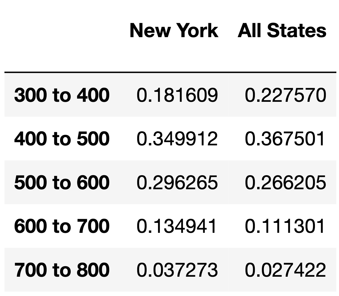
Now, suppose we’re interested in comparing the verbal score distribution of students who took the SAT in New York in 2015 to the verbal score distribution of all students who took the SAT in 2015.
The DataFrame scores_2015, shown in its entirety below,
contains the verbal section score distributions of students in New York
in 2015 and for all students in 2015.
What type of test is being proposed above?
Hypothesis test
Permutation test
Answer: Hypothesis test
One way to think about “standard” hypothesis tests is that they test whether a given sample – in this case, the verbal score distribution of New York students in 2015 – looks like it was drawn from a given population – here, the verbal score distribution of all students in 2015. That’s what’s happening here.
The average score on this problem was 87%.
Suppose \vec{a} = \begin{bmatrix} a_1 &
a_2 & ... & a_n \end{bmatrix}^T and \vec{b} = \begin{bmatrix} b_1 & b_2 & ...
& b_n \end{bmatrix}^T are both vectors containing proportions
that add to 1 (e.g. \vec{a} could be
the "New York" column above and \vec{b} could be the
"All States" column above). As we’ve seen before, the TVD
is defined as follows:
\text{TVD}(\vec{a}, \vec{b}) = \frac{1}{2} \sum_{i = 1}^n \left| a_i - b_i \right|
The TVD is not the only metric that can quantify the distance between two categorical distributions. Here are three other possible distance metrics:
\text{dis1}(\vec{a}, \vec{b}) = \vec{a} \cdot \vec{b} = a_1b_1 + a_2b_2 + ... + a_nb_n
\text{dis2}(\vec{a}, \vec{b}) = \frac{\vec{a} \cdot \vec{b}}{|\vec{a} | | \vec{b} |} = \frac{a_1b_1 + a_2b_2 + ... + a_nb_n}{\sqrt{a_1^2 + a_2^2 + ... + a_n^2} \sqrt{b_1^2 + b_2^2 + ... + b_n^2}}
\text{dis3}(\vec{a}, \vec{b}) = 1 - \frac{\vec{a} \cdot \vec{b}}{|\vec{a} | | \vec{b} |}
Of the above three possible distance metrics, only one of them has the same range as the TVD (i.e. the same minimum possible value and the same maximum possible value) and has the property that smaller values correspond to more similar vectors. Which distance metric is it?
\text{dis1}
\text{dis2}
\text{dis3}
Answer: \text{dis3}
Let’s look at the options carefully:
The average score on this problem was 75%.
The function state_perm is attempting to implement a
test of the null hypothesis that the distributions of mean math section
scores between 2005 and 2015 for two states are drawn from the same
population distribution.
def state_perm(states):
    if len(states) != 2:
        raise ValueError(f"Expected 2 elements, got {len(states)}")

    def calc_test_stat(df):
        return df.groupby("State")["Math"].mean().abs().diff().iloc[-1]

    states = sat.loc[sat["State"].isin(states), ["State", "Math"]]

    test_stats = []
    for _ in range(10000):
        states["State"] = np.random.permutation(states["State"])
        test_stat = calc_test_stat(states)
        test_stats.append(test_stat)

    obs = calc_test_stat(states)
    return (np.array(test_stats) >= obs).mean()
Suppose we call state_perm(["California", "Washington"])
and see 0.514.
What test statistic is being used in the above call to
state_perm?
\text{mean Washington score } - \text{mean California score}
\text{mean California score } - \text{mean Washington score}
\big|\text{mean Washington score } - \text{mean California score} \big|
Answer: Option 1
Lets take a deeper look at calc_test_stat(df).
The function first calculates the mean math scores in each state.
Although the .abs() method is applied, it is redundant at
this stage since no differences have been computed yet. The key
operation is .diff(), which computes the difference between
the mean scores of the two states. Since groupby sorts states
alphabetically, it subtracts the mean score of California (appearing
first) from Washington (appearing second). The final expression
df.groupby("State")["Math"].mean().abs().diff().iloc[-1]
thus represents mean Washington score − mean California score.
The average score on this problem was 27%.
There is exactly one issue with the implementation of
state_perm. In exactly one sentence,
identify the issue and state how you would fix it.
Hint: The issue is not with the implementation
of the function calc_test_stat.
Answer: Since we are permuting in-place on the
states DataFrame, we must calculate the observed test
statistic before we permute.
The average score on this problem was 81%.
To prepare for the verbal component of the SAT, Nicole decides to read research papers on data science. While reading these papers, she notices that there are many citations interspersed that refer to other research papers, and she’d like to read the cited papers as well.
In the papers that Nicole is reading, citations are formatted in the
verbose numeric style. An excerpt from one such paper is stored
in the string s below.
s = '''
In DSC 10 [3], you learned about babypandas, a strict subset
of pandas [15][4]. It was designed [5] to provide programming
beginners [3][91] just enough syntax to be able to perform
meaningful tabular data analysis [8] without getting lost in
100s of details.
'''
We decide to help Nicole extract citation numbers from papers. Consider the following four extracted lists.
list1 = ['10', '100']
list2 = ['3', '15', '4', '5', '3', '91', '8']
list3 = ['10', '3', '15', '4', '5', '3', '91', '8', '100']
list4 = ['[3]', '[15]', '[4]', '[5]', '[3]', '[91]', '[8]']
list5 = ['1', '0', '3', '1', '5', '4', '5', '3',
         '9', '1', '8', '1', '0', '0']
For each expression below, select the list it evaluates to, or select “None of the above.”
re.findall(r'\d+', s)
list1
list2
list3
list4
list5
None of the above
Answer: list3
This regex pattern \d+ matches one or more digits
anywhere in the string. It doesn’t concern itself with the context of
the digits, whether they are inside brackets or not. As a result, it
extracts all sequences of digits in s, including '10',
'3', '15', '4', '5',
'3', '91', '8', and
'100', which together form list3. This is
because \d+ greedily matches all contiguous digits,
capturing both the citation numbers and any other numbers present in the
text.
The average score on this problem was 81%.
re.findall(r'[\d+]', s)
list1
list2
list3
list4
list5
None of the above
Answer: list5
This pattern [\d+] is slightly misleading because the
square brackets are used to define a character class, and the plus sign
inside is treated as a literal character, not as a quantifier. However,
since there are no plus signs in s, this detail does not
affect the outcome. The character class \d matches any
digit, so this pattern effectively matches individual digits throughout
the string, resulting in list5. This list contains every
single digit found in s, separated as individual string
elements.
The average score on this problem was 31%.
re.findall(r'\[(\d+)\]', s)
list1
list2
list3
list4
list5
None of the above
Answer: list2
This pattern is specifically designed to match digits that are
enclosed in square brackets. The \[(\d+)\] pattern looks
for a sequence of one or more digits \d+ inside square
brackets []. The parentheses capture the digits as a group,
excluding the brackets from the result. Therefore, it extracts just the
citation numbers as they appear in s, matching
list2 exactly. This method is precise for extracting
citation numbers from a text formatted in the verbose numeric style.
The average score on this problem was 80%.
re.findall(r'(\[\d+\])', s)
list1
list2
list3
list4
list5
None of the above
Answer: list4
Similar to the previous explanation but with a key difference: the
entire pattern of digits within square brackets is captured, including
the brackets themselves. The pattern \[\d+\] specifically
searches for sequences of digits surrounded by square brackets, and the
parentheses around the entire pattern ensure that the match includes the
brackets. This results in list4, which contains all the
citation markers found in s, preserving the brackets to
clearly denote them as citations.
The average score on this problem was 91%.
After taking the SAT, Nicole wants to check the College Board’s website to see her score. However, the College Board recently updated their website to use non-standard HTML tags and Nicole’s browser can’t render it correctly. As such, she resorts to making a GET request to the site with her scores on it to get back the source HTML and tries to parse it with BeautifulSoup.
Suppose soup is a BeautifulSoup object instantiated
using the following HTML document.
<college>Your score is ready!</college>

<sat verbal="ready" math="ready">
  Your percentiles are as follows:
  <scorelist listtype="percentiles">
    <scorerow kind="verbal" subkind="per">
      Verbal: <scorenum>84</scorenum>
    </scorerow>
    <scorerow kind="math" subkind="per">
      Math: <scorenum>99</scorenum>
    </scorerow>
  </scorelist>
  And your actual scores are as follows:
  <scorelist listtype="scores">
    <scorerow kind="verbal"> Verbal: <scorenum>680</scorenum> </scorerow>
    <scorerow kind="math"> Math: <scorenum>800</scorenum> </scorerow>
  </scorelist>
</sat>Which of the following expressions evaluate to "verbal"?
Select all that apply.
soup.find("scorerow").get("kind")
soup.find("sat").get("ready")
soup.find("scorerow").text.split(":")[0].lower()
[s.get("kind") for s in soup.find_all("scorerow")][-2]
soup.find("scorelist", attrs={"listtype":"scores"}).get("kind")
None of the above
Answer: Option 1, Option 3, Option 4
Correct options:
<scorerow> element and
retrieves its "kind" attribute, which is
"verbal" for the first <scorerow>
encountered in the HTML document.<scorerow> tag,
retrieves its text ("Verbal: 84"), splits this text by “:”,
and takes the first element of the resulting list
("Verbal"), converting it to lowercase to match
"verbal"."kind" attributes for all
<scorerow> elements. The second to last (-2) element
in this list corresponds to the "kind" attribute of the
first <scorerow> in the second
<scorelist> tag, which is also
"verbal".Incorrect options:
<sat> tag, which does not exist as an attribute."kind" attribute from a
<scorelist> tag, but <scorelist>
does not have a "kind" attribute.
The average score on this problem was 90%.
Consider the following function.
def summer(tree):
    if isinstance(tree, list):
        total = 0
        for subtree in tree:
            for s in subtree.find_all("scorenum"):
                total += int(s.text)
        return total
    else:
        return sum([int(s.text) for s in tree.find_all("scorenum")])
For each of the following values, fill in the blanks to assign
tree such that summer(tree) evaluates to the
desired value. The first example has been done for you.
84 tree = soup.find("scorerow")183 tree = soup.find(__a__)1480 tree = soup.find(__b__)899 tree = soup.find_all(__c__)Answer: a: "scorelist", b:
"scorelist", attrs={"listtype":"scores"}, c:
"scorerow", attrs={"kind":"math"}
soup.find("scorelist") selects the first
<scorelist> tag, which includes both verbal and math
percentiles (84 and 99). The function
summer(tree) sums these values to get 183.
The average score on this problem was 92%.
This selects the <scorelist> tag with
listtype="scores", which contains the actual scores of
verbal (680) and math (800). The function sums
these to get 1480.
The average score on this problem was 92%.
This selects all <scorerow>elements with
kind="math", capturing both the percentile
(99) and the actual score (800). Since tree is
now a list, summer(tree) iterates through each
<scorerow> in the list, summing their
<scorenum> values to reach 899.
The average score on this problem was 91%.
Consider the following list of tokens.
tokens = ["is", "the", "college", "board", "the", "board", "of", "college"]Recall, a uniform language model is one in which each
unique token has the same chance of being sampled.
Suppose we instantiate a uniform language model on tokens.
The probability of the sentence “the college board is” — that is, P(\text{the college board is}) — is of the
form \frac{1}{a^b}, where a and b are
both positive integers.
What are a and b?
Answer: a = 5, b = 4
In a uniform language model, each unique token has the same chance of being sampled. Given the list of tokens, there are 5 unique tokens: [“is”, “the”, “college”, “board”, “of”]. The probability of sampling any one token is \frac{1}{5}. For a sentence of 4 tokens (“the college board is”), the probability is \frac{1}{5^4} because each token is independently sampled. Thus, a = 5 and b = 4.
The average score on this problem was 70%.
Recall, a unigram language model is one in which the chance that a
token is sampled is equal to its observed frequency in the list of
tokens. Suppose we instantiate a unigram language model on
tokens. The probability P(\text{the college board is}) is of the form
\frac{1}{c^d}, where c and d are
both positive integers.
What are c and d?
Answer: (c, d) = (2, 9) or (8, 3)
In a unigram language model, the probability of sampling a token is proportional to its frequency in the token list. The frequencies are: “is” = 1, “the” = 2, “college” = 2, “board” = 2, “of” = 1. The sentence “the college board is” has probabilities \frac{2}{8}, \frac{2}{8}, \frac{2}{8}, \frac{1}{8} for each word respectively, when considering the total number of tokens (8). The combined probability is \frac{2}{8} \cdot \frac{2}{8} \cdot \frac{2}{8} \cdot \frac{1}{8} = \frac{8}{512} = \frac{1}{2^9} or, simplifying, \frac{1}{8^3} since 512 = 8^3. Therefore, c = 2 and d = 9 or c = 8 and d = 3, depending on how you represent the fraction.
The average score on this problem was 68%.
For the remainder of this question, consider the following five sentences.
"of the college board the""the board the board the""board the college board of""the college board of college""board the college board is"Recall, a bigram language model is an N-gram model with N=2. Suppose we instantiate a bigram language
model on tokens. Which of the following sentences of length
5 is the most likely to be sampled?
Sentence 1
Sentence 2
Sentence 3
Sentence 4
Sentence 5
Answer: Sentence 4
Remember, our corpus was:
["is", "the", "college", "board", "the", "board", "of", "college"]In order for a sentence to be sampled, it must be made up of bigrams
that appeared in the corpus. This automatically rules out Sentence 1,
because "of the" never appears in the corpus and Sentence
5, because "board is" never appears in the corpus.
Then, let’s compute the probabilities of the other three sentences:
Sentence 2:
\begin{align*} P(\text{the board the board the}) &= P(\text{the}) \cdot P(\text{board | the}) \cdot P(\text{the | board}) \cdot P(\text{board | the}) \cdot P(\text{the | board}) \\ &= \frac{2}{8} \cdot \frac{1}{2} \cdot \frac{1}{2} \cdot \frac{1}{2} \cdot \frac{1}{2} \\ &= \frac{1}{64} \end{align*}
Sentence 3:
\begin{align*} P(\text{board the college board of}) &= P(\text{board}) \cdot P(\text{the | board}) \cdot P(\text{college | the}) \cdot P(\text{board | college}) \cdot P(\text{of | board}) \\ &= \frac{2}{8} \cdot \frac{1}{2} \cdot \frac{1}{2} \cdot 1 \cdot \frac{1}{2} \\ &= \frac{1}{32}\end{align*}
Sentence 4:
\begin{align*} P(\text{the college board of college}) &= P(\text{the}) \cdot P(\text{college | the}) \cdot P(\text{board | college}) \cdot P(\text{of | board}) \cdot P(\text{college | of}) \\ &= \frac{2}{8} \cdot \frac{1}{2} \cdot 1 \cdot \frac{1}{2} \cdot 1 \\ &= \frac{1}{16} \end{align*}
Thus, Sentence 4 is most likely to be sampled.
The average score on this problem was 72%.
For your convenience, we repeat the same five sentences again below.
"of the college board the""the board the board the""board the college board of""the college board of college""board the college board is"Suppose we create a TF-IDF matrix, in which there is one row for each sentence and one column for each unique word. The value in row i and column j is the TF-IDF of word j in sentence i. Note that since there are 5 sentences and 5 unique words across all sentences, the TF-IDF matrix has 25 total values.
Is there a column in the TF-IDF matrix in which all values are 0?
Yes
No
Answer: Yes
Recall,
\text{tf-idf}(t, d) = \text{term frequency}(t, d) \cdot \text{inverse document frequency}(t)
In the context of TF-IDF, if a word appears in every sentence, its inverse document frequency (IDF) would be \log(\frac{5}{5}) = 0. Since a word’s TF-IDF in a document is its TF (term frequency) in that document multiplied by its IDF, if the word’s IDF is 0, it’s TF-IDF is also 0. Since “the” appears in all five sentences, its IDF is zero, leading to a column of zeros in the TF-IDF matrix for “the”.
The average score on this problem was 49%.
In which of the following sentences is “college” the word with the highest TF-IDF?
Sentence 1
Sentence 2
Sentence 3
Sentence 4
Sentence 5
Answer: Sentence 4
Remember, the IDF of a word is the same for all documents, since $(t) = ( )$. This means that the sentence where “college” is the word with the highest TF-IDF is the same as the sentence where “college” is the word with the highest TF, or term frequency. Sentence 4 is the only sentence where “college” appears twice; in all other sentences, “college” appears at most once. (Since all of these sentences have the same length, we know that if “college” appears more times in Sentence 4 than it does in other sentences, then “college”’s term frequency in Sentence 4, \frac{2}{5}, is also larger than in any other sentence.) As such, the answer is Sentence 4.
The average score on this problem was 95%.
As an alternative to TF-IDF, Yuxin proposes the DF-ITF, or “document frequency-inverse term frequency”. The DF-ITF of term t in document d is defined below:
\text{df-itf}(t, d) = \frac{\text{\# of documents in which $t$ appears}}{\text{total \# of documents}} \cdot \log \left( \frac{\text{total \# of words in $d$}}{\text{\# of occurrences of $t$ in $d$}} \right)
Fill in the blank: The term t in document d that best summarizes document d is the term with ____.
the largest DF-ITF in document d
the smallest DF-ITF in document d
Answer: the smallest DF-IDF in document d
The key idea behind TF-IDF, as we learned in class, is that t is a good summary of d if t occurs commonly in d but rarely across all documents.
When t occurs often in d, then \frac{\text{\# of occurrences of $t$ in $d$}}{\text{total \# of words in $d$}} is large, which means \frac{\text{total \# of words in $d$}}{\text{\# of occurrences of $t$ in $d$}} and hence \log \left( \frac{\text{total \# of words in $d$}}{\text{\# of occurrences of $t$ in $d$}} \right) is small.
Similarly, if t is rare across all documents, then \frac{\text{\# of documents in which $t$ appears}}{\text{total \# of documents}} is small.
Putting the above two pieces together, we have that \text{df-itf}(t, d) is small when t occurs commonly in d but rarely overall, which means that the term t that best summarizes d is the term with the smallest DF-IDF in d.
The average score on this problem was 90%.
We decide to build a classifier that takes in a state’s demographic information and predicts whether, in a given year:
The state’s mean math score was greater than its mean verbal score (1), or
the state’s mean math score was less than or equal to its mean verbal score (0).
The simplest possible classifier we could build is one that predicts the same label (1 or 0) every time, independent of all other features.
Consider the following statement:
If a > b, then the constant classifier that
maximizes training accuracy predicts 1 every time; otherwise, it
predicts 0 every time.
For which combination of a and b is the
above statement not guaranteed to be true?
Note: Treat sat as our training set.
Option 1:
a = (sat['Math'] > sat['Verbal']).mean()
b = 0.5
Option 2:
a = (sat['Math'] - sat['Verbal']).mean()
b = 0
Option 3:
a = (sat['Math'] - sat['Verbal'] > 0).mean()
b = 0.5
Option 4:
a = ((sat['Math'] / sat['Verbal']) > 1).mean() - 0.5
b = 0
Option 1
Option 2
Option 3
Option 4
Answer: Option 2
Conceptually, we’re looking for a combination of a and
b such that when a > b, it’s true that
in more than 50% of states, the "Math" value is
larger than the "Verbal" value. Let’s look at all
four options through this lens:
sat['Math'] > sat['Verbal'] is a Series of
Boolean values, containing True for all states where the
"Math" value is larger than the "Verbal" value
and False for all other states. The mean of this series,
then, is the proportion of states satisfying this criteria, and since
b is 0.5, a > b is
True only when the bolded condition above is
True.sat['Math'] / sat['Verbal'] is a Series that
contains values greater than 1 whenever a state’s "Math"
value is larger than its "Verbal" value and less than or
equal to 1 in all other cases. As in the other options that work,
(sat['Math'] / sat['Verbal']) > 1 is a Boolean Series
with True for all states with a larger "Math"
value than "Verbal" values; a > b compares
the proportion of True values in this Series to 0.5. (Here,
p - 0.5 > 0 is the same as p > 0.5.)Then, by process of elimination, Option 2 must be the correct option
– that is, it must be the only option that doesn’t
work. But why? sat['Math'] - sat['Verbal'] is a Series
containing the difference between each state’s "Math" and
"Verbal" values, and .mean() computes the mean
of these differences. The issue is that here, we don’t care about
how different each state’s "Math" and
"Verbal" values are; rather, we just care about the
proportion of states with a bigger "Math" value than
"Verbal" value. It could be the case that 90% of states
have a larger "Math" value than "Verbal"
value, but one state has such a big "Verbal" value that it
makes the mean difference between "Math" and
"Verbal" scores negative. (A property you’ll learn about in
future probability courses is that this is equal to the difference in
the mean "Math" value for all states and the mean
"Verbal" value for all states – this is called the
“linearity of expectation” – but you don’t need to know that to answer
this question.)
The average score on this problem was 58%.
Suppose we train a classifier, named Classifier 1, and it achieves an accuracy of \frac{5}{9} on our training set.
Typically, root mean squared error (RMSE) is used as a performance metric for regression models, but mathematically, nothing is stopping us from using it as a performance metric for classification models as well.
What is the RMSE of Classifier 1 on our training set? Give your answer as a simplified fraction.
Answer: \frac{2}{3}
An accuracy of \frac{5}{9} means that the model is such that out of 9 values, 5 are labeled correctly. By extension, this means that 4 out of 9 are not labeled correctly as 0 or 1.
Remember, RMSE is defined as
\text{RMSE} = \sqrt{\frac{1}{n} \sum_{i = 1}^n (y_i - H(x_i))^2}
where y_i represents the ith actual value and H(x_i) represents the ith prediction. Here, y_i is either 0 or 1 and $H(x_i) is also either 0 or 1. We’re told that \frac{5}{9} of the time, y_i and H(x_i) are the same; in those cases, (y_i - H(x_i))^2 = 0^2 = 0. We’re also told that \frac{4}{9} of the time, y_i and H(x_i) are different; in those cases, (y_i - H(x_i))^2 = 1. So,
\text{RMSE} = \sqrt{\frac{5}{9} \cdot 0 + \frac{4}{9} \cdot 1} = \sqrt{\frac{4}{9}} = \frac{2}{3}
The average score on this problem was 55%.
While Classifier 1’s accuracy on our training set is \frac{5}{9}, its accuracy on our test set is \frac{1}{4}. Which of the following scenarios is most likely?
Classifier 1 overfit to our training set; we need to increase its complexity.
Classifier 1 overfit to our training set; we need to decrease its complexity.
Classifier 1 underfit to our training set; we need to increase its complexity.
Classifier 1 underfit to our training set; we need to decrease its complexity.
Answer: Option 2
Since the accuracy of Classifier 1 is much higher on the dataset used to train it than the dataset it was tested on, it’s likely Classifer 1 overfit to the training set because it was too complex. To fix the issue, we need to decrease its complexity, so that it focuses on learning the general structure of the data in the training set and not too much on the random noise in the training set.
The average score on this problem was 86%.
For the remainder of this question, suppose we train another classifier, named Classifier 2, again on our training set. Its performance on the training set is described in the confusion matrix below. Note that the columns of the confusion matrix have been separately normalized so that each has a sum of 1.
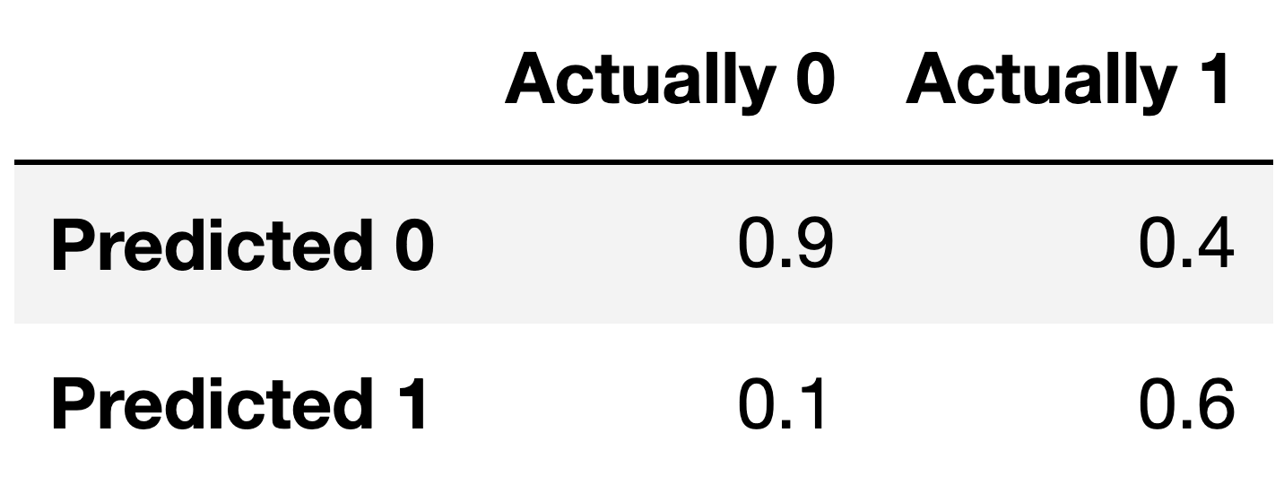
Suppose conf is the DataFrame above. Which of the
following evaluates to a Series of length 2 whose only unique value is
the number 1?
conf.sum(axis=0)
conf.sum(axis=1)
Answer: Option 1
Note that the columns of conf sum to 1 – 0.9 + 0.1 = 1, and 0.4 + 0.6 = 1. To create a Series with just
the value 1, then, we need to sum the columns of conf,
which we can do using conf.sum(axis=0).
conf.sum(axis=1) would sum the rows of
conf.
The average score on this problem was 81%.
Fill in the blank: the ___ of Classifier 2 is guaranteed to be 0.6.
precision
recall
Answer: recall
The number 0.6 appears in the bottom-right corner of
conf. Since conf is column-normalized, the
value 0.6 represents the proportion of values in the second column that
were predicted to be 1. The second column contains values that were
actually 1, so 0.6 is really the proportion of values that were
actually 1 that were predicted to be 1, that is, \frac{\text{actually 1 and predicted
1}}{\text{actually 1}}. This is the definition of recall!
If you’d like to think in terms of true positives, etc., then remember that: - True Positives (TP) are values that were actually 1 and were predicted to be 1. - True Negatives (TN) are values that were actually 0 and were predicted to be 0. - False Positives (FP) are values that were actually 0 and were predicted to be 1. - False Negatives (FN) are values that were actually 1 and were predicted to be 0.
Recall is \frac{\text{TP}}{\text{TP} + \text{FN}}.
The average score on this problem was 77%.
For your convenience, we show the column-normalized confusion matrix from the previous page below. You will need to use the specific numbers in this matrix when answering the following subpart.
Suppose a fraction \alpha of the labels in the training set are actually 1 and the remaining 1 - \alpha are actually 0. The accuracy of Classifier 2 is 0.65. What is the value of \alpha?
Hint: If you’re unsure on how to proceed, here are some guiding questions:
Suppose the number of y-values that are actually 1 is A and that the number of y-values that are actually 0 is B. In terms of A and B, what is the accuracy of Classifier 2? Remember, you’ll need to refer to the numbers in the confusion matrix above.
What is the relationship between A, B, and \alpha? How does it simplify your calculation for the accuracy in the previous step?
Answer: \frac{5}{6}
Here is one way to solve this problem:
accuracy = \frac{TP + TN}{TP + TN + FP + FN}
Given the values from the confusion matrix:
accuracy = \frac{0.6 \cdot \alpha + 0.9
\cdot (1 - \alpha)}{\alpha + (1 - \alpha)}
accuracy = \frac{0.6 \cdot \alpha + 0.9 - 0.9
\cdot \alpha}{1}
accuracy = 0.9 - 0.3 \cdot \alpha
Therefore:
0.65 = 0.9 - 0.3 \cdot \alpha
0.3 \cdot \alpha = 0.9 - 0.65
0.3 \cdot \alpha = 0.25
\alpha = \frac{0.25}{0.3}
\alpha = \frac{5}{6}
The average score on this problem was 61%.
Let’s continue with the premise from the previous question. That is, we will aim to build a classifier that takes in demographic information about a state from a particular year and predicts whether or not the state’s mean math score is higher than its mean verbal score that year.
In honor of the
rotisserie
chicken event on UCSD’s campus a few weeks ago, sklearn
released a new classifier class called
ChickenClassifier.
ChickenClassifiers have many hyperparameters, one of
which is height. As we increase the value of
height, the model variance of the resulting
ChickenClassifier also increases.
First, we consider the training and testing accuracy of a
ChickenClassifier trained using various values of
height. Consider the plot below.
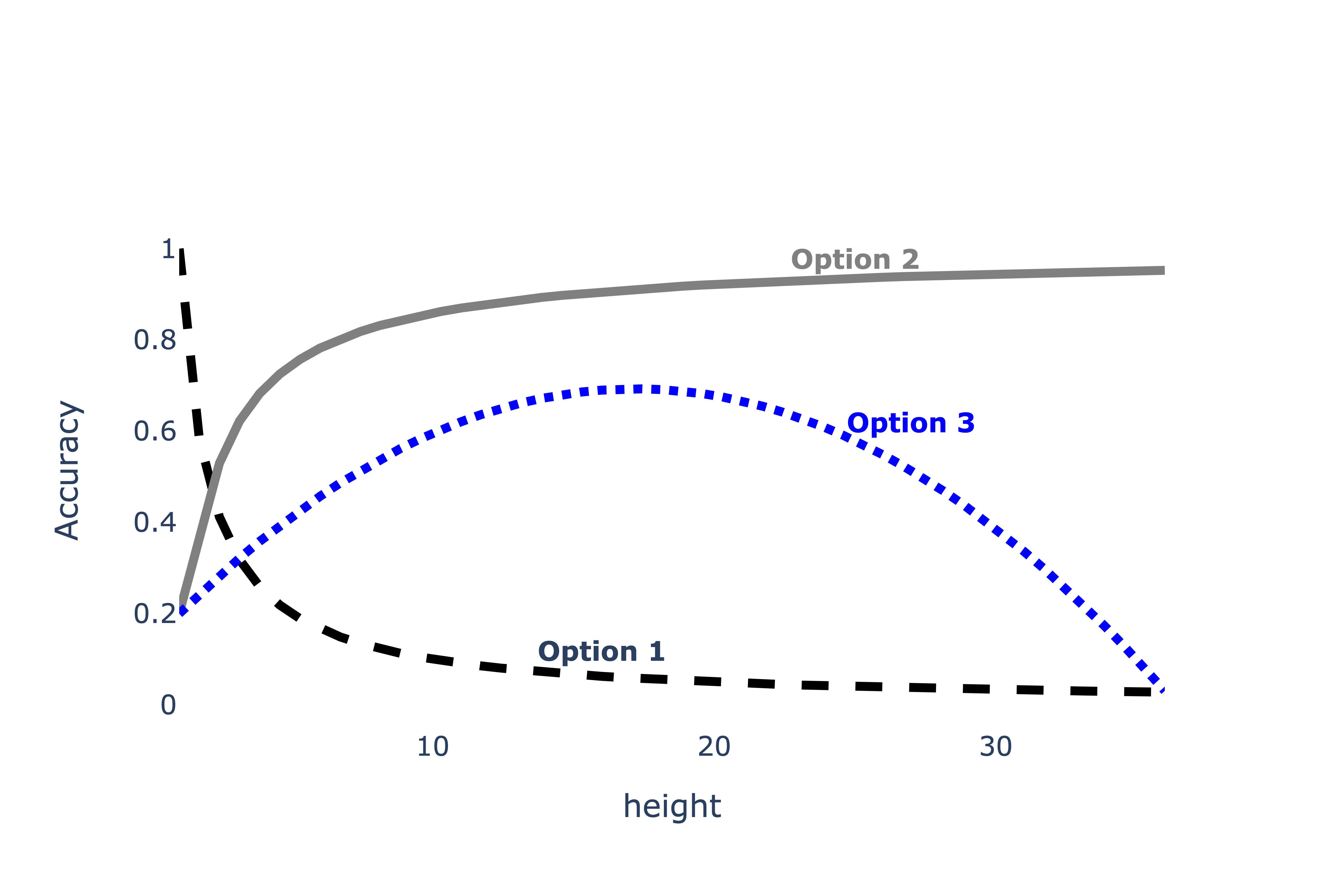
Which of the following depicts training accuracy
vs. height?
Option 1
Option 2
Option 3
Which of the following depicts testing accuracy
vs. height?
Option 1
Option 2
Option 3
Answer: Option 2 depicts training accuracy
vs. height; Option 3 depicts testing accuract
vs. height
We are told that as height increases, the model variance
(complexity) also increases.
As we increase the complexity of our classifier, it will do a better
job of fitting to the training set because it’s able to “memorize” the
patterns in the training set. As such, as height increases,
training accuracy increases, which we see in Option 2.
However, after a certain point, increasing height will
make our classifier overfit too closely to our training set and not
general enough to match the patterns in other similar datasets, meaning
that after a certain point, increasing height will actually
decrease our classifier’s accuracy on our testing set. The only option
that shows accuracy increase and then decrease is Option 3.
The average score on this problem was 75%.
ChickenClassifiers have another hyperparameter,
color, for which there are four possible values:
"yellow", "brown", "red", and
"orange". To find the optimal value of color,
we perform k-fold cross-validation with
k=4. The results are given in the table
below.
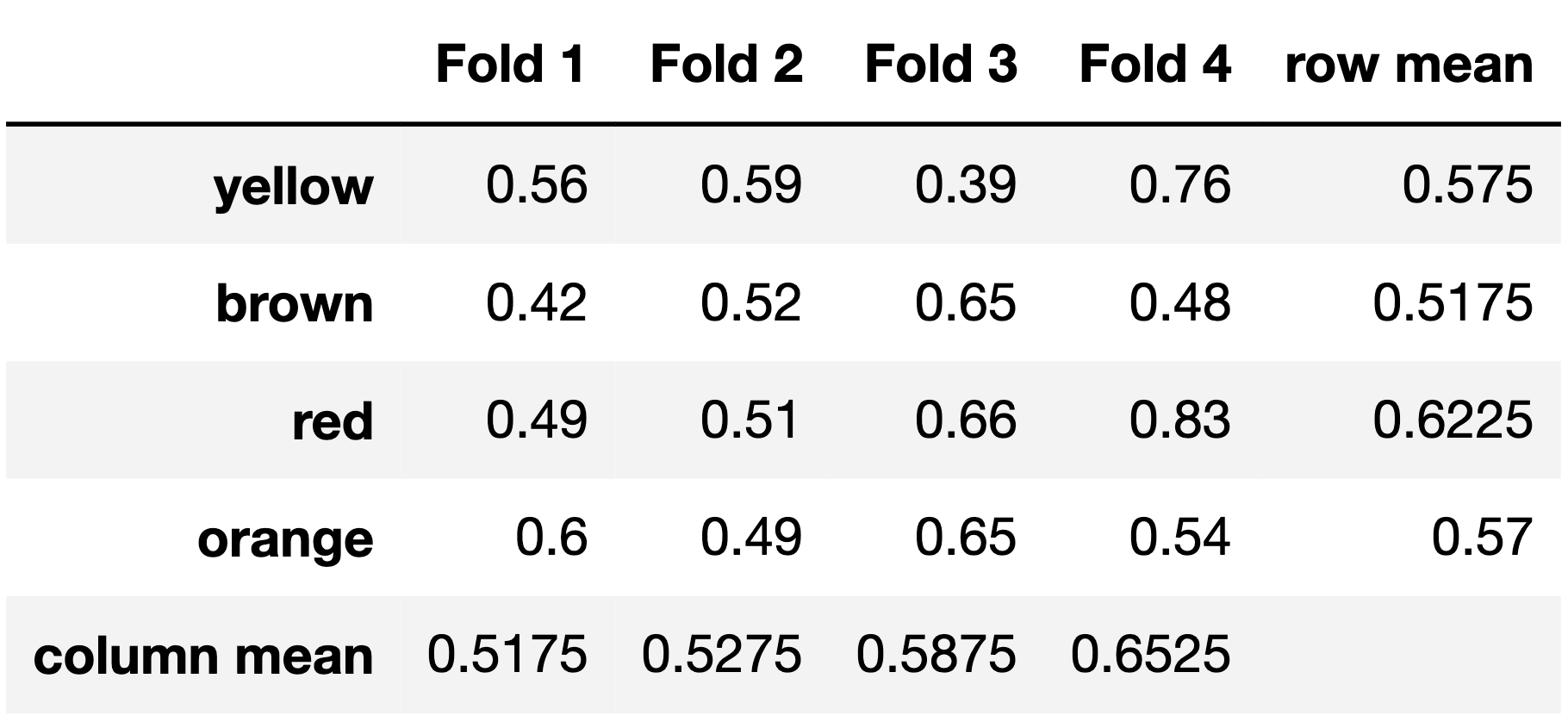
Which value of color has the best average validation
accuracy?
"yellow"
"brown"
"red"
"orange"
Answer: "red"
From looking at the results of the k-fold cross validation, we see that the color red has the highest, and therefore the best, validation accuracy as it has the highest row mean (across all 4 folds).
The average score on this problem was 91%.
True or False: It is possible for a hyperparameter value to have the best average validation accuracy across all folds, but not have the best validation accuracy in any one particular fold.
True
False
Answer: True
An example is shown below:
| color | Fold 1 | Fold 2 | Fold 3 | Fold 4 | average |
|---|---|---|---|---|---|
| color 1 | 0.8 | 0 | 0 | 0 | 0.2 |
| color 2 | 0 | 0.6 | 0 | 0 | 0.15 |
| color 3 | 0 | 0 | 0.1 | 0 | 0.025 |
| color 4 | 0 | 0 | 0 | 0.2 | 0.05 |
| color 5 | 0.7 | 0.5 | 0.01 | 0.1 | 0.3275 |
In the example, color 5 has the highest average validation accuracy across all folds, but is not the best in any one fold.
The average score on this problem was 94%.
Now, instead of finding the best height and best
color individually, we decide to perform a grid search that
uses k-fold cross-validation to find
the combination of height and color with the
best average validation accuracy.
For the purposes of this question, assume that:
height and h_2 possible
values of color.Consider the following three subparts:
Choose from the following options.
k
\frac{k}{n}
\frac{n}{k}
\frac{n}{k} \cdot (k - 1)
h_1h_2k
h_1h_2(k-1)
\frac{nh_1h_2}{k}
None of the above
Answer: A: Option 3 (\frac{n}{k}), B: Option 6 (h_1h_2(k-1)), C: Option 8 (None of the above)
The training set is divided into k folds of equal size, resulting in k folds with size \frac{n}{k}.
The average score on this problem was 66%.
For each combination of hyperparameters, row 5 is k - 1 times for training and 1 time for validation. There are h_1 \cdot h_2 combinations of hyperparameters, so row 5 is used for training h_1 \cdot h_2 \cdot (k-1) times.
The average score on this problem was 76%.
Building off of the explanation for the previous subpart, row 5 is used for validation 1 times for each combination of hyperparameters, so the correct expression would be h_1 \cdot h_2, which is not a provided option.
The average score on this problem was 69%.
One piece of information that may be useful as a feature is the
proportion of SAT test takers in a state in a given year that qualify
for free lunches in school. The Series lunch_props contains
8 values, each of which are either "low",
"medium", or "high". Since we can’t use
strings as features in a model, we decide to encode these strings using
the following Pipeline:
# Note: The FunctionTransformer is only needed to change the result
# of the OneHotEncoder from a "sparse" matrix to a regular matrix
# so that it can be used with StandardScaler;
# it doesn't change anything mathematically.
pl = Pipeline([
    ("ohe", OneHotEncoder(drop="first")),
    ("ft", FunctionTransformer(lambda X: X.toarray())),
    ("ss", StandardScaler())
])
After calling pl.fit(lunch_props),
pl.transform(lunch_props) evaluates to the following
array:
array([[ 1.29099445, -0.37796447],
       [-0.77459667, -0.37796447],
       [-0.77459667, -0.37796447],
       [-0.77459667,  2.64575131],
       [ 1.29099445, -0.37796447],
       [ 1.29099445, -0.37796447],
       [-0.77459667, -0.37796447],
       [-0.77459667, -0.37796447]])
and pl.named_steps["ohe"].get_feature_names() evaluates
to the following array:
array(["x0_low", "x0_med"], dtype=object)Fill in the blanks: Given the above information, we can conclude that
lunch_props has (a) value(s) equal to
"low", (b) value(s) equal to
"medium", and (c) value(s) equal to
"high". (Note: You should write one positive integer in
each box such that the numbers add up to 8.)
What goes in the blanks?
Answer: 3, 1, 4
The first column of the transformed array corresponds to the
standardized one-hot-encoded low column. There are 3 values
that are positive, which means there are 3 values that were originally
1 in that column pre-standardization. This means that 3 of
the values in lunch_props were originally
"low".
The second column of the transformed array corresponds to the
standardized one-hot-encoded med column. There is only 1
value in the transformed column that is positive, which means only 1 of
the values in lunch_props was originally
"medium".
The Series lunch_props has 8 values, 3 of which were
identified as "low" in subpart 1, and 1 of which was
identified as "medium" in subpart 2. The number of values
being "high" must therefore be 8
- 3 - 1 = 4.
The average score on this problem was 73%.