← return to practice.dsc80.com
Instructor(s): Suraj Rampure
This exam was administered in-person. The exam was closed-notes, except students were allowed to bring a single two-sided cheat sheet. No calculators were allowed. Students had 50 minutes to take this exam.
Welcome to the Midterm Exam for DSC 80 in Spring 2022!
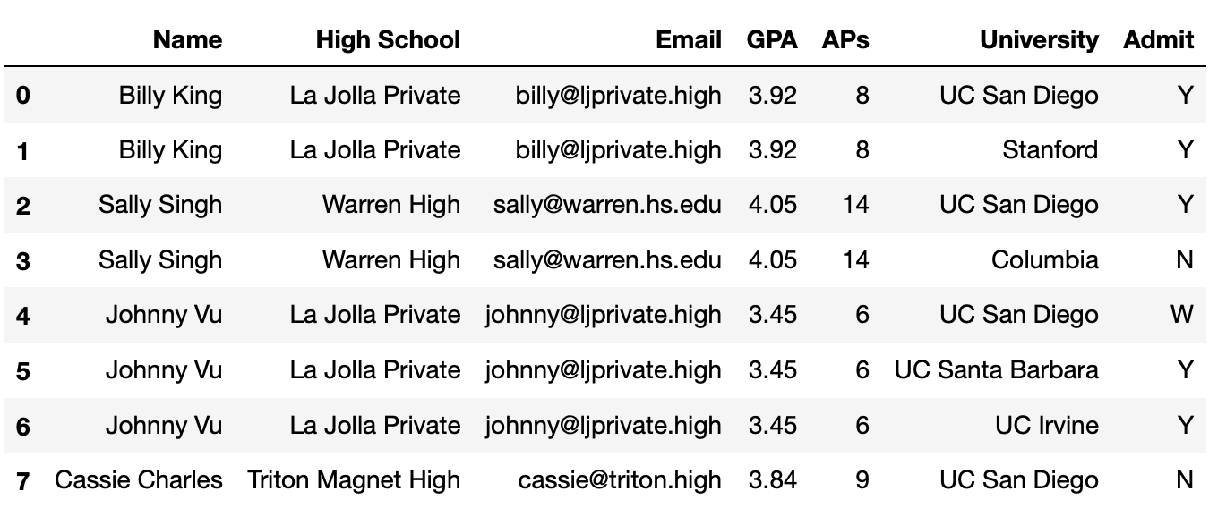
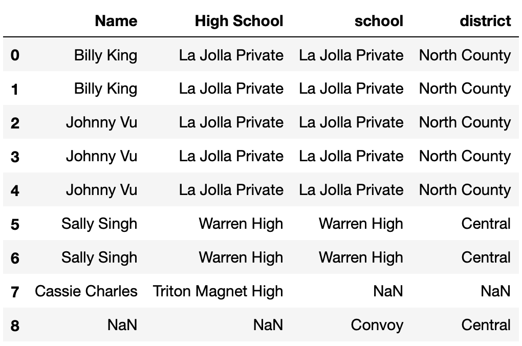
Throughout this exam, we will be using the following DataFrame
students, which contains various information about high
school students and the university/universities they applied to.
The columns are:
'Name' (str): the name of the student.'High School' (str): the High School that the student
attended.'Email' (str): the email of the student.'GPA' (float): the GPA of the student.'AP' (int): the number of AP exams that the student
took.'University' (str): the name of the university that the
student applied to.'Admit' (str): the acceptance status of the student
(where ‘Y’ denotes that they were accepted to the university and ‘N’
denotes that they were not).The rows of 'student' are arranged in no particular
order. The first eight rows of 'student' are shown above
(though 'student' has many more rows than pictured
here).
What kind of variable is "APs"?
Quantitative discrete
Quantitative continuous
Qualitative ordinal
Qualitative nominal
Answer: Quantitative discrete
Since we can count the number of "APs" a student is
enrolled in, it is clearly a quantitative variable. Also note that the
number of "APs" a student is enrolled in has to be a whole
number, hence it is a quantitative discrete variable.
The average score on this problem was 97%.
Because we can sort universities by admit rate,
"University" is a qualitative ordinal variable.
True
False
Answer: False
In order for a categorical variable to be ordinal, there must be some inherent order to the categories. We can always sort a categorical column based on some other column, but that doesn’t make the categories themselves ordinal. For instance, we can sort colors based on how much King Triton likes them, but that doesn’t make colors ordinal!
The average score on this problem was 79%.
Write a single line of code that evaluates to the most common value
in the "High School" column of students, as a
string. Assume there are no ties.
Answer:
students["High School"].value_counts().idxmax()
or
students.groupby("High School")["Name"].count().sort_values().index[-1]
The average score on this problem was 89%.
Fill in the blank so that the result evaluates to a Series indexed by
"Email" that contains a list of the
universities that each student was admitted to. If a
student wasn’t admitted to any universities, they should have an empty
list.
students.groupby("Email").apply(_____)What goes in the blank?
Answer:
lambda df: df.loc[df["Admit"] == "Y", "University"].tolist()
The average score on this problem was 53%.
Which of the following blocks of code correctly assign
max_AP to the maximum number of APs taken by a student who
was rejected by UC San Diego?
Option 1:
cond1 = students["Admit"] == "N"
cond2 = students["University"] == "UC San Diego"
max_AP = students.loc[cond1 & cond2, "APs"].sort_values().iloc[-1]
Option 2:
cond1 = students["Admit"] == "N"
cond2 = students["University"] == "UC San Diego"
d3 = students.groupby(["University", "Admit"]).max().reset_index()
max_AP = d3.loc[cond1 & cond2, "APs"].iloc[0]
Option 3:
p = students.pivot_table(index="Admit",
                            columns="University",
                            values="APs",
                            aggfunc="max")
max_AP = p.loc["N", "UC San Diego"]
Option 4:
# .last() returns the element at the end of a Series it is called on
groups = students.sort_values(["APs", "Admit"]).groupby("University")
max_AP = groups["APs"].last()["UC San Diego"]
Select all that apply. There is at least one correct option.
Option 1
Option 2
Option 3
Option 4
Answer: Option 1 and Option 3
Option 1 works correctly, it is probably the most straightforward
way of answering the question. cond1 is True
for all rows in which students were rejected, and cond2 is
True for all rows in which students applied to UCSD. As
such, students.loc[cond1 & cond2] contains only the
rows where students were rejected from UCSD. Then,
students.loc[cond1 & cond2, "APs"].sort_values() sorts
by the number of "APs" taken in increasing order, and
.iloc[-1] gets the largest number of "APs"
taken.
Option 2 doesn’t work because the lengths of cond1
and cond2 are not the same as the length of
d3, so this causes an error.
Option 3 works correctly. For each combination of
"Admit" status ("Y", "N",
"W") and "University" (including UC San
Diego), it computes the max number of "APs". The usage of
.loc["N", "UC San Diego"] is correct too.
Option 4 doesn’t work. It currently returns the maximum number of
"APs" taken by someone who applied to UC San Diego; it does
not factor in whether they were admitted, rejected, or
waitlisted.
The average score on this problem was 85%.
Currently, students has a lot of repeated information —
for instance, if a student applied to 10 universities, their GPA appears
10 times in students.
We want to generate a DataFrame that contains a single row for each
student, indexed by "Email", that contains their
"Name", "High School", "GPA", and
"APs".
One attempt to create such a DataFrame is below.
students.groupby("Email").aggregate({"Name": "max",
                                        "High School": "mean",
                                        "GPA": "mean",
                                        "APs": "max"})
There is exactly one issue with the line of code above. In one sentence, explain what needs to be changed about the line of code above so that the desired DataFrame is created.
Answer: The problem right now is that aggregating
High School by mean doesn’t work since you can’t aggregate a column with
strings using "mean". Thus changing it to something that
works for strings like "max" or "min" would
fix the issue.
The average score on this problem was 79%.
Consider the following snippet of code.
pivoted = students.assign(Admit=students["Admit"] == "Y") \
                    .pivot_table(index="High School",
                                columns="University",
                                values="Admit",
                                aggfunc="sum")
Some of the rows and columns of pivoted are shown
below.
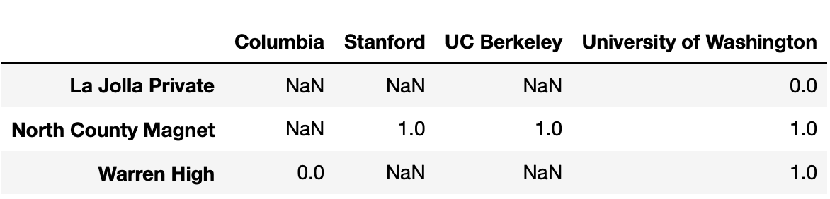
No students from Warren High were admitted to Columbia or Stanford.
However,
pivoted.loc["Warren High", "Columbia"] and
pivoted.loc["Warren High", "Stanford"] evaluate to
different values. What is the reason for this difference?
Some students from Warren High applied to Stanford, and some others applied to Columbia, but none applied to both.
Some students from Warren High applied to Stanford but none applied to Columbia.
Some students from Warren High applied to Columbia but none applied to Stanford.
The students from Warren High that applied to both Columbia and Stanford were all rejected from Stanford, but at least one was admitted to Columbia.
When using pivot_table, pandas was not able
to sum strings of the form "Y", "N", and
"W", so the values in pivoted are
unreliable.
Answer: Option 3
pivoted.loc["Warren High", "Stanford"] is
NaN because there were no rows in students in
which the "High School" was "Warren High" and
the "University" was "Stanford", because
nobody from Warren High applied to Stanford. However,
pivoted.loc["Warren High", "Columbia"] is not
NaN because there was at least one row in
students in which the "High School" was
"Warren High" and the "University" was
"Columbia". This means that at least one student from
Warren High applied to Columbia.
Option 3 is the only option consistent with this logic.
The average score on this problem was 93%.
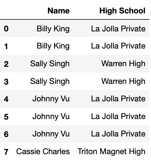
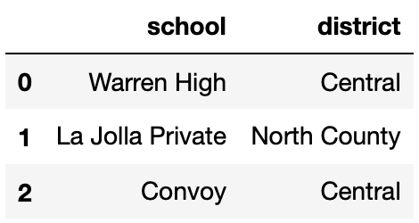
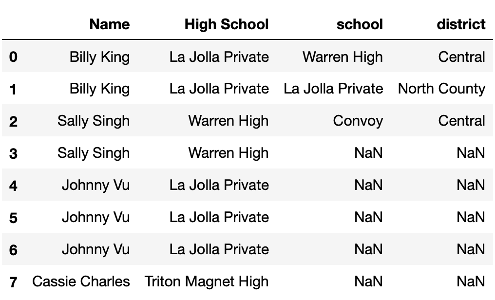
Define small_students to be the DataFrame with 8 rows
and 2 columns shown directly below, and define districts to
be the DataFrame with 3 rows and 2 columns shown below
small_students.
Consider the DataFrame merged, defined below.
merged = small_students.merge(districts,
                                left_on="High School",
                                right_on="school",
how="outer")How many total NaN values does merged
contain? Give your answer as an integer.
Answer: 4
merged is shown below.
The average score on this problem was 13%.
Consider the DataFrame concatted, defined below.
concatted = pd.concat([small_students, districts], axis=1)How many total NaN values does concatted
contain? Give your answer as an integer.
Hint: Draw out what concatted looks like. Also,
remember that the default axis argument to
pd.concat is axis=0.
Answer: 10
concatted is shown below.
The average score on this problem was 76%.
Let’s consider admissions at UC San Diego and UC Santa Barbara for two high schools in particular.
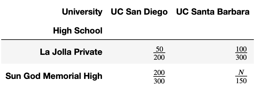
For instance, the above table tells us that 200 students from La Jolla Private applied to UC San Diego, and 50 were admitted.
What is the largest possible integer value of N such that:
UC Santa Barbara has a strictly higher admit rate for both La Jolla Private and Sun God Memorial High individually, but
UC San Diego has a strictly higher admit rate overall?
Answer: 124
Let’s consider the two conditions separately.
First, UC Santa Barbara needs to have a higher admit rate for both high schools. This is already true for La Jolla Private (\frac{100}{300} > \frac{50}{200}); for Sun God Memorial High, we just need to ensure that \frac{N}{150} > \frac{200}{300}. This means that N > 100.
Now, UC San Diego needs to have a higher admit rate overall. The UC San Diego admit rate is \frac{50+200}{200+300} = \frac{250}{500} = \frac{1}{2}, while the UC Santa Barbara admit rate is \frac{100 + N}{450}. This means that we must require that \frac{1}{2} = \frac{225}{450} > \frac{100+N}{450}. This means that 225 > 100 + N, i.e. that N < 125.
So there are two conditions on N: N > 100 and N < 125. The largest integer N that satisfies these conditions is N=124, which is the final answer.
The average score on this problem was 72%.
Valentina has over 1000 students. When a student signs up for
Valentina’s college counseling, they must provide a variety of
information about themselves and their parents. Valentina keeps track of
all of this information in a table, with one row per student. (Note that
this is not the students DataFrame from
earlier in the exam.)
Valentina asks each her students for the university that their
parents attended for undergrad. The "father’s university"
column of Valentina’s table contains missing values. Valentina believes
that values in this column are missing because not all students’ fathers
attended university.
According to Valentina’s interpretation, what is the missingness
mechanism of "father’s university"?
Missing by design
Not missing at random
Missing at random
Missing completely at random
Answer: Not missing at random
Per Valentina’s interpretation, the reason for the missingness in the
"father’s university" column is that not all fathers
attended university, and hence they opted not to fill out the survey.
Here, the likelihood that values are missing depends on the values
themselves, so the data are NMAR.
The average score on this problem was 81%.
The "mother’s phone number" column of Valentina’s table
contains missing values. Valentina knows for a fact that all of her
students’ mothers have phone numbers. She looks at her dataset and draws
the following visualization, relating the missingness of
"mother’s phone number" to "district" (the
school district that the student’s family lives in):
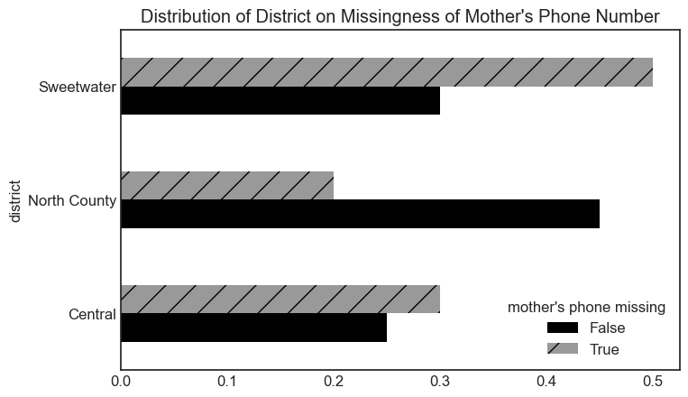
Given just the above information, what is the missingness mechanism
of "mother’s phone number"?
Missing by design
Not missing at random
Missing at random
Missing completely at random
Answer: Missing at random
Here, the distribution of "district" is different when
"mother’s phone number" is missing and when
"mother’s phone number" is present (the two distributions
plotted look quite different). As such, we conclude that the missingness
of "mother’s phone number" depends on
"district", and hence the data are MAR.
The average score on this problem was 88%.
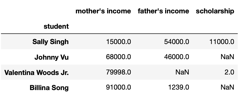
UC Hicago, a new private campus of the UC, has an annual tuition of $80,000. UC Hicago states that if an admitted student’s parents’ combined income is under $80,000, they will provide that student a scholarship for the difference.
Valentina keeps track of each student’s parents’ incomes along with the scholarship that UC Hicago promises them in a table. The first few rows of her table are shown below.
Given just the above information, what is the missingness mechanism
of "scholarship"?
Missing by design
Not missing at random
Missing at random
Missing completely at random
Answer: Missing by design
Here, the data are missing by design because you can 100% of the time
predict whether a "scholarship" will be missing by looking
at the "mother’s income" and "father’s income"
columns. If the sum of "mother’s income" and
"father’s income" is at least $80,000,
"scholarship" will be missing; otherwise, it will not be
missing.
The average score on this problem was 88%.
Consider the following pair of hypotheses.
Null hypothesis: The average GPA of UC San Diego admits from La Jolla Private is equal to the average GPA of UC San Diego admits from all schools.
Alternative hypothesis: The average GPA of UC San Diego admits from La Jolla Private is less than the average GPA of UC San Diego admits from all schools.
What type of test is this?
Hypothesis test
Permutation test
Answer: Hypothesis test
Here, we are asking if one sample is a random sample of a known population. While this may seem like a permutation test in which we compare two samples, there is really only one sample here — the GPAs of admits from La Jolla Private. To simulate new data, we sample from the distribution of all GPAs.
Note that this is similar to the bill lengths on Torgersen Island example from Lecture 6 (in Spring 2022, at least).
The average score on this problem was 75%.
Which of the following test statistics would be appropriate to use in this test? Select all valid options.
La Jolla Private mean GPA
Difference between La Jolla Private mean GPA and overall mean GPA
Absolute difference between La Jolla Private mean GPA and overall mean GPA
Total variation distance (TVD)
Kolmogorov-Smirnov (K-S) statistic
Answer: Option 1 and 2
In hypothesis tests where we test to see if a sample came from a larger distribution, we often use the sample mean as the test statistic (again, see the Torgersen Island bill lengths example from Lecture 12). Hence, the La Jolla Private mean GPA is a valid option.
Note that in this hypothesis test, we will simulate new data by generating random samples, each one being the same size as the number of applications from La Jolla Private. The overall mean GPA will not change on each simulation, as it is a constant. Hence, Option 2 reduces to Option 1 minus a constant, which purely shifts the distribution of the test statistic and the observed statistic horizontally but does not change their relative positions to one another. Hence, the difference between the La Jolla Private mean GPA and overall mean GPA is also a valid test statistic.
Option 3 is not valid because our alternative hypothesis has a direction (that the mean GPA of La Jolla Private admits is less than the mean GPA of all admits). The absolute difference would be appropriate for a directionless alternative hypothesis, e.g. that the mean GPA of La Jolla Private admits is different than the mean GPA of all admits.
Option 4 doesn’t work because we are not dealing with categorical distributions.
Option 5 doesn’t work because we are not running a permutation test to test if two samples come from the underlying population distribution; rather, here we are testing if one sample comes from a larger population (and our hypotheses explicitly mentioned the mean).
The average score on this problem was 81%.
Consider the following pair of hypotheses.
Null hypothesis: The distribution of admitted, waitlisted, and rejected students at UC San Diego from Warren High is equal to the distribution of admitted, waitlisted, and rejected students at UC San Diego from La Jolla Private.
Alternative hypothesis: The distribution of admitted, waitlisted, and rejected students at UC San Diego from Warren High is different from the distribution of admitted, waitlisted, and rejected students at UC San Diego from La Jolla Private.
What type of test is this?
Hypothesis test
Permutation test
Answer: Permutation test
There are two relevant distributions at play here:
The distribution of admit/waitlist/reject proportions at Warren High.
The distribution of admit/waitlist/reject proportions at La Jolla Private.
To generate new data under the null, we need to shuffle the group labels, i.e. randomly assign students to groups.
The average score on this problem was 89%.
Which of the following test statistics would be appropriate to use in this test? Select all valid options.
Warren High admit rate
Difference between Warren High and La Jolla Private admit rates
Absolute difference between Warren High and La Jolla Private admit rates
Total variation distance (TVD)
Kolmogorov-Smirnov (K-S) statistic
Answer: Option 4
The two distributions described in 11(a) are categorical, and the TVD is the only test statistic that measures the "distance" between two categorical distributions.
The average score on this problem was 79%.
After getting bored of working with her students, Valentina decides to experiment with different ways of simulating data for the following pair of hypotheses:
Null hypothesis: The coin is fair.
Alternative hypothesis: The coin is biased in favor of heads.
As her test statistic, Valentina uses the number of heads. She
defines the 2-D array A as follows:
# .flatten() reshapes from 50 x 2 to 1 x 100
A = np.array([
    np.array([np.random.permutation([0, 1]) for _ in range(50)]).flatten()
    for _ in range(3000)
])
She also defines the 2-D array B as follows:
# .flatten() reshapes from 50 x 2 to 1 x 100
B = np.array([
    np.array([np.random.choice([0, 1], 2) for _ in range(50)]).flatten()
    for _ in range(3000)
])
Below, we see a histogram of the distribution of her test statistics.
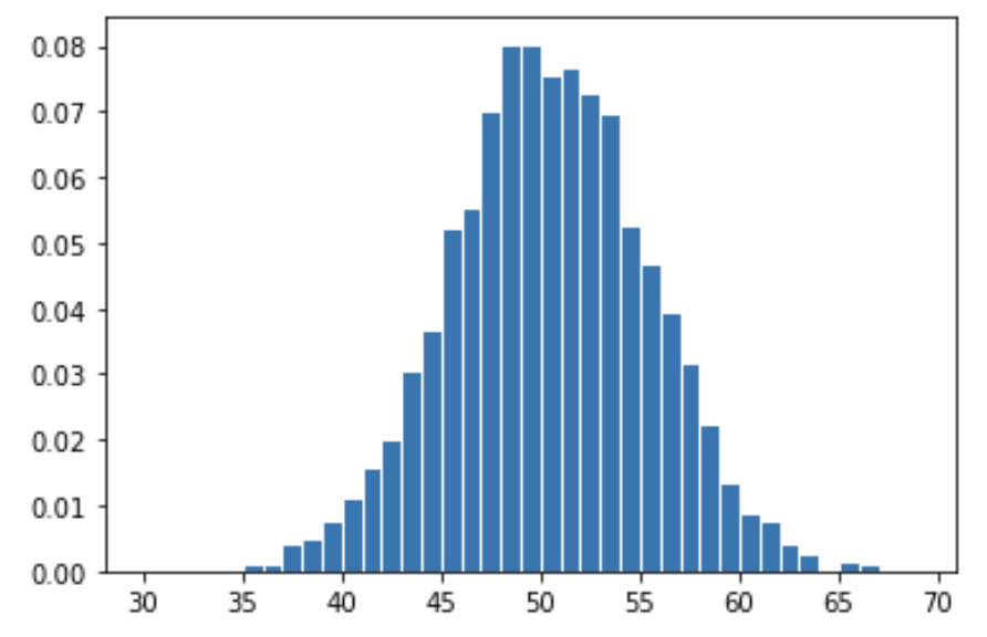
Which one of the following arrays are visualized above?
A.sum(axis=1)
B.sum(axis=1)
Answer: Option 2
Note that arr.sum(axis=1) takes the sum of each
row of arr.
The difference comes down to the behavior of
np.random.permutation([0, 1]) and
np.random.choice([0, 1]).
Each call to np.random.permutation([0, 1]) will either
return array([0, 1]) or array([1, 0]) — one
head and one tail. As a result, each row of A will consist
of 50 1s and 50 0s, and so the sum of each row of A will be
exactly 50. If we drew a histogram of this distribution, it would be a
single spike at the number 50.
On the other hand, each call to
np.random.choice([0, 1], 2) could either return
array([0, 0]), array([0, 1]),
array([1, 0]), or array([1, 1]). Each of these
are returned with equal probabilities. In effect,
np.random.choice([0, 1], 2) flips a fair coin twice, so
[np.random.choice([0, 1], 2) for _ in range(50)] flips a
fair coin 100 times. When we take the sum of each row of B,
we will get the number of heads in 100 coin flips; the histogram drawn
is consistent with this interpretation.
The average score on this problem was 83%.