
← return to practice.dsc80.com
Instructor(s): Sam Lau
This exam was administered in-person. The exam was closed-notes, except students were allowed to bring a single two-sided notes sheet. No calculators were allowed. Students had 80 minutes to take this exam.
Fill in Python code below so that the last line of each part
evaluates to each desired result, assuming that the following tables are
both stored as pandas DataFrames. You may not use
for or while loops in any answer for this
question. Only the first few rows are shown for each table.
The df table (left) records what people ate in kilograms
(kg) on each date in 2023. For example, the first row records that Sam
ate 0.2 kg of Ribeye on Jan 1, 2023. The foods table
(right) records the carbon dioxide (CO2) emissions it takes to produce
each kind of food. For example, the first row in the foods
table shows that growing 1 kg of mung beans produces 0.1 kg of CO2.
Find the total kg of food eaten for each day and each person in
df as a Series.
df.groupby(____)[____].sum()Answer:
df.groupby(['date', 'name'])['weight'].sum()
To satisfy “each day and each person”, we need to group by both the
'date' and 'name' columns by passing them in
as a list. Then to get “kg of food eaten”, we must select the
'weight' column with the second blank. The
sum() method then will get the “total” amount as a Series
(where you have 'date' and 'name' as indices
and the sum as the value).
The average score on this problem was 87%.
Find all the rows in df where Tina was the person
eating.
df.____Answer:
df.loc[df['name'] == 'Tina']
We can use the loc accessor to select the rows from
df under a specific condition, where rows satisfying the
condition as True will be selected. In this case, to get
the rows where “Tina was the person eating”, our conditional is when a
value from the column df['name'] is equal to the string
'Tina'.
The average score on this problem was 67%.
Find all the unique people who did not eat any food containing the word “beans”.
def foo(x):
    return ____

df.groupby(____).____(foo)['name'].unique()Answer:
def foo(x):
    return x['food'].str.contains('beans').sum() == 0

df.groupby('name').filter(foo)['name'].unique()
To solve this, we start with the bottom line since without it we
don’t know what the argument x is in foo(x).
Since we want to find “the unique people”, we will group by
'name' to get to the per-individual level. Then, since we
want to only keep the rows corresponding to certain groups, we can use
the filter function. Since we pass foo into
filter, we can now work on the foo function
knowing x will be a group of df when
aggregated by 'name' (all the rows belonging to a single
name).
To find people who ate food containing the word 'beans',
we need to find the column of the food they ate: x['food'].
Then we can recall that pandas has built-in string
manipulation methods that can be used on every element of a Series by
calling .str.name_of_method(). In this case, to find the
string 'beans' we will use
.str.contains('beans'). At this point, we have a Boolean
Series representing for one person, which meals they ate contained the
word 'beans' – an element in this Series is
True if the corresponding meal contained
'beans' and False otherwise.
We want to ensure that they didn’t eat any 'beans',
which would be true if all of the values in this Boolean Series are
False, i.e. if the sum of the Boolean Series (since
Trues are counted as 1 and Falses are counted
as 0) is 0. This explains the == 0 at the end.
The code then selects the 'name' column and returns an
array with its unique values, giving us the unique people who didn’t eat
any 'beans'.
The average score on this problem was 39%.
Create a copy of df tht has one extra column called
'words that contains the number of words for each value in
the 'food' column. Assume that words are separated by one
space character. For example, “Pinto beans” has two words.
def f(x):
    return ____

df.assign(____)Answer:
def f(x):
    return len(x.split())

df.assign(words = df['food'].apply(f))
Like the problem before, we need to start with the bottom line before
working on f(x) so that we can determine what the parameter
x represents. We are given the assign method,
which we know will create a new column with format
assign(column_name=values). We are given that our new
column name is 'words', so now we just need to get the
values: the number of words for each value in the 'food'
column.
Knowing we have a helper function f, we can use the
apply method on the 'food' column
df['food'] to pass each value in food through
f. Then, we can use f to calculate the number
of words per value in 'food', where the input to
f (that is, x) is a single value. Since we are
given that words are separated by whitespace, we can just call
x.split() to get a list with each word in its own index.
The len of that list is therefore the count of words.
The average score on this problem was 82%.
Find the total kg of CO2 produced by each person in
df. If a food in df doesn’t have a matching
value in foods, assume that the food generates 100 kg of CO2 per kg of food.
df2 = df.merge(foods, ____)
(df2.assign(____).groupby('name')['c'].sum()) Answer:
df2 = df.merge(foods, left_on='food', right_index=True, how = 'left')
(df2.assign(c=df2['weight'] * df2['co2/kg'].fillna(100).groupby('name')['c'].sum())
To begin, we are merging df and foods as
df2, but we need to figure out how. There are multiple ways
to do this, so your answer might not match exactly what we have. We can
see that the way to merge so we get the 'co2/kg' for each
food is to merge the 'food' column of df with
the index of foods. Since df is on the left,
we pass in left_on='food'. Since foods is on
the right and we are merging on the index not a column, we pass in
right_index=True as well. Then, we are told “if a food
doesn’t have a matching value in foods, assume that the
food generates 100 kg of CO2
per kg of food. This means we can’t use the default inner join as this
will drop non-matching values. Instead, we want to keep everything in
the df table, so we say how='left' to do a
left join.
Now that we have df2 that has all the columns of
df as well as a column of the 'co2/kg' for
each row, we can calculate the CO2 production per person. We
see that we are given code that groups the dataframe by person name,
selects some column 'c' that isn’t in df2 yet,
and then sums the values. This seems to handle the
total kg of CO2 per person
by calling and groupby('name') and the .sum()
aggregation method. That tells us we need to make a new column in
df2 named 'c', representing the kg of
CO2 per meal/row. We are already given the
assign method in the code, so we know that in that blank we
need c = [some Series containing CO2 weights]. We have the
'weight' and 'co2/kg' columns in
df2, so multiplying these would give us the end
CO2 for 'c'. This looks like
df2['weight'] * df2['co2/kg'].
Finally, we must recall that we are expected to handle the case where
there is no matching value in the merge. Since we are doing a left join,
we keep every value in df and might fill in some values of
foods with NaN values. That means
df2['co2/kg'] needs to have NaN values
replaced with 100, and that can be done with
fillna(100). That makes our final solution
c=df2['weight'] * df2['co2/kg'].fillna(100).
The average score on this problem was 65%.
For this question, we’ll continue using the df and
foods tables form Question 1. Dyaln and Giorgia want to compare their
CO_2 emissions. They added a new column
called 'bean' to df that contains
True if the food was a bean (e.g. “Pinto beans”) and
False otherwise. Then, they compute the following pivot
table:
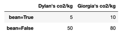
Each entry in the pivot table is the average CO_2 emissions for Dylan and Giorgia per kg of food they ate (CO_2/kg) for both bean and non-bean foods.
Suppose that overall, Dylan produced an average of 41 CO_2/kg of food he ate, while Giorgia produced an average of 38 CO_2/kg. Determine whether each statement is definitely true (T), definitely false (F), or whether more information is needed (M) beyond this information and the pivot table above.
Answer:
A. T
B. M
C. T
D. M
A. Definitely True. Simpson’s paradox is the case where grouped
data and ungrouped data show different trends. In this case, the
ungrouped data shown by the table – that is, when we
look at CO_2/kg emissions
separately for when when 'bean' is
True and when 'bean' is False –
give the appearance that Giogia’s CO_2/kg is greater than Dylan’s. However, the
grouped data – that is, the overall
data – tells us that Dylan’s CO_2/kg is
greater.
B. More info needed. Since this problem only deals with the proportion of CO_2/kg, we cannot know anything about the actual kg amounts. 41 CO_2/kg can be 41 CO_2 in 1 kg of eaten food, or 410 CO_2 in 10 kg of eaten food.
C. Definitely True. This is definitely be true because we see
that Giorgia’s overall average CO_2/kg
is lower than Dylan’s, even though her separate amounts in both
categories are greater. This is because both Dylan and Giorgia had
different proportions of their food be made up of 'bean'
foods. In this case, since the case where 'bean' is
True produces less CO_2/kg, Giorgia must have a higher proportion
of her food being 'bean' foods in order to average out with
a lower CO_2/kg than Dylan.
D. More info needed. Similar to part B, we only know about the CO_2/kg proportion, and not the actual amounts. Even though Dylan has a higher average CO_2/kg output, if he ate less kg of food than Giorgia he may emit less kg of CO_2 overall.
The average score on this problem was 75%.
Dylan and Giorgia want to figure out exactly when Simpson’s paradox occurs for their data. Suppose that 0.2 proportion of Dylan’s food was bean foods. What range of proportions for Giorgia’s bean food would cause Simpson’s paradox to occur? Show your work in the space below, then write your final answer in the blanks at the bottom of the page. Your final answers should be between 0 and 1. Leave your answers as simplified fractions.
Between ____ and ____
Answer: Between \frac{39}{70} and 1
First, we solve for the proportions that make the average overall
CO_2/kg the same for Dylan and Giorgia
as our threshold value. Since we are finding Giorgia’s range of
proportions, we will form our equation from her table column and set it
equal to Dylan’s average production:
41 = 10B_{True} + 80B_{False}
Where B_{True} represents the
proportion of foods that Giorgia eats that are 'bean' (that
is, Giorgia’s 'bean' is True proportion) and
B_{False} represents the proportion of
foods that Giorgia eats that are not 'bean' (that is,
Giorgia’s 'bean' is False proportion).
We also know that these two must add to 1, so:
1 = B_{True} + B_{False} \\\implies B_{False} = 1 - B_{True}
We can now plug this in to our first equation to get:
41 = 10B_{True} + 80(1 - B_{True}) \\... \\B_{True} =\frac{39}{70}
Next we find whether Simpson’s paradox occurs above or below this
value where the two are equal. Since the ungrouped data shows Giorgia’s
CO_2/kg emissions are greater than
Dylan’s for both the case where 'bean' is True
(10 > 5) and where 'bean' is False (80 >
10), we want to find the range of B_{True} that results in an overall average
that is lower than 41.
We can see that plugging in B_{True}=1
gives: 10(1) + 80(0) = 10
so our solution will be between \frac{39}{70} and 1.
The average score on this problem was 59%.
The donkeys table contains data from a research study
about donkey health. The researchers measured the attributes of 544 donkeys. The next day, they selected
30 donkeys to reweigh. The first few
rows of the donkeys table are shown below (left), and the
table contains the following columns (right):

What is the feature type of each column in donkeys? For
each column below, answer discrete continuous, continuous, ordinal, or
nominal.
'id': ____'BCS': ____'Age': ____'Weight': ____'WeightAlt': ____Answer:
'id': Nominal'BCS': Ordinal'Age': Ordinal'Weight': Continuous'WeightAlt': ContinuousLet’s look one by one.
'id': Nominal. This is qualitative data. While each
'id' has a number such as 01 or 02,
these numbers are not ordered to signify any id is “greater” than
another, and arithmetic doesn’t make sense with them.'BCS': Ordinal. This is qualitative data as
'BCS' is an interpretive score representing “emaciated” to
“obese”. The data is ordered as it follows the scale mentioned
prior.'Age': Ordinal. This is qualitative data since the age
is bucketed as “<2”, “2-5”, and so on. The data is ordered as “<2”
is younger than “2-5”, so this is also a scale of age.'Weight': Continuous. This is quantitative since weight
is a numeric measurement. It is continuous because there is no given
restriction on the values the weight can take on.'WeightAlt': Continuous. This is quantitative since
weight is a numeric measurement. It is continuous because there is no
given restriction on the values the weight can take on. Note that null
values do not change the feature type of this variable.Note that discrete continuous is not a real feature type!
The average score on this problem was 66%.
Consider the following scenarios for how the researchers chose the
30 donkeys to reweigh. In each
scenario, select if the missing mechanism for the
'WeightAlt' column is NMAR, MAR, or MCAR.
Note: Although the missing data are missing by design from the perspective of the original researchers, since we can’t directly recover the missing values from our other data, we can treat the missing data as NMAR, MAR, or MCAR.
'Weight' values to reweigh.'BCS score of 4 or
greater.i as a number drawn uniformly at
random between 0 and 514, then reweighed the donkeys in
donkeys.iloc[i:i+30].'WeightAlt' except for the 30 lowest values.Answer:
Again, let’s look one by one.
'WeightAlt' depend on the 'Weight' column
since we select the 30 largest.'WeightAlt' depend on the 'BCS' column since
we choose from those with a score of 4
or greater.i = 0, but index 29 could
be chosen if i is any value between 0 and 29, so
it has a higher probability of being chosen. The original solution was
MCAR as we did not account for edge case of i being small,
but it is technically MAR. Credit was given for either answer.'Weight', and so they depend on the column itself.
The average score on this problem was 86%.
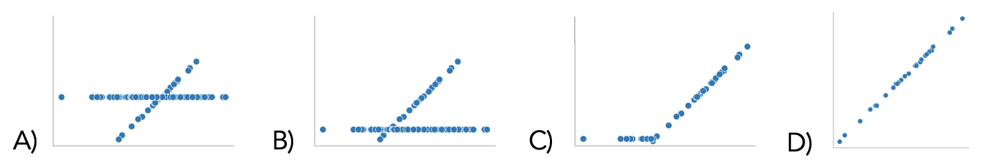
In this question, we will continue to work with the
donkeys dataset from Problem 3. The first few rows of the table column
descriptions are shown again below for convenience.
For this question, assume that the researchers chose the 30 donkeys to reweigh by drawing a
simple random sample of 30 underweight
donkeys: donkeys with BCS values of 1,
1.5, or 2. The researchers weighed these
30 donkeys one day later and stored the
results in the 'WeightAlt'.
Which of the following shows the scatter plot of
'WeightAlt' - 'Weight' on the y-axis and
'Weight' on the x-axis? Assume that missing values are not
plotted.

Answer: D
We are measuring the difference in weight from just one day on the y-axis, which means we can’t expect any noticeable pattern of weight gain or loss no matter the original weight of the donkey. Therefore, a random scatterplot makes sense. Options A through C all suggest that the single-day weight change correlates with the starting weight, which is not a good assumption.
The average score on this problem was 53%.
Suppose we use mean imputation to fill in the missing values in
'WeightAlt'. Select the scatter plot
'WeightAlt' on 'Weight' after imputation.
Answer: A
Note we are now plotting 'Weight' on the y-axis, not the
difference of 'WeightAlt' - 'Weight'. Therefore, it makes
sense that we would have 30 data points
with a positive slope as the initial weight and re-weight are likely
very similar.
Then, mean imputation is the process of filling in missing values with the average of the non-missing values. Therefore, all missing values will be the same, and should be at the center of the sloped line since the line is roughly evenly distributed.
The average score on this problem was 67%.
Alan wants to see whether donkeys with 'BCS' >= 3 have larger 'Weight' values on
average compared to donkeys that have 'BCS' < 3. Select all the possible test
statistics that Alan could use to conduct this hypothesis test.
Let \mu_1 be the mean weight of donkeys
with 'BCS' >= 3 and
\mu_2 be the mean weight of donkeys
with 'BCS' < 3.
Answer: B and C
The average score on this problem was 75%.
To generate a single sample under his null hypothesis, Alan should: -
A. Resample 744 donkeys with
replacement from donkeys. - B. Resample 372 donkeys with replacement from
donkeys with 'BCS' < 3, and another 372 donkeys with 'BCS' >=
3. - C. Randomly permute the
'Weight' column.
Answer: C)
The null hypothesis is “Donkeys with 'BCS' >= 3 have the same
'Weight' values on average compared to donkeys that have
'BCS' < 3”. Under the
null hypothesis, we should have similar results with a shuffled dataset.
Options A and B shuffle with replacement (bootstrapping), while option C
shuffles without replacement (permutation is done without replacement).
Bootstrapping is generally used to estimate confidence intervals, while
permutation tests are a kind of hypothesis test. In this case, we are
performing a hypothesis test, so we want to permute the
'Weight' column.
The average score on this problem was 54%.
Doris wants to use multiple imputation to fill in the missing values
in 'WeightAlt'. She knows that 'WeightAlt' is
MAR conditional on 'BCS' and 'Age', so she
will perform multiple imputation conditional on 'BCS' and
'Age' - each missing value will be filled in with vlaues
from a random 'WeightAlt' value from a donkey with
the same 'BCS' and 'Age'. Assume that
all 'BCS' and 'Age' cmbinations have observed
WegihtAlt values. Fill in the blanks in the code below to
estimate the median of 'WeightAlt' using multiple
imputation conditional on 'BCS' and 'Age' with
100 repetitions. A function
impute is also partially filled in for you, and you should
use it in your answer.
def impute(col):
    col = col.copy()
    n = ____
    fill = np.random.choice(____)
    col[____] = fill
    return col
results = []
for i in range(____):
    imputed = (donkeys.____(____)['WeightAlt'].____(____))
results.append(imputed.median())Answer:
def impute(col):
    col = col.copy()
    n = col.isna().sum()
    fill = np.random.choice(col.dropna(), n)
    col[col.isna()] = fill
    return col
results = []
for i in range(100):
    imputed = (donkeys.groupby(['BCS', 'Age'])['WeightAlt'].transform(impute))
    results.append(imputed.median())
We start with the bottom five blanks as we are not sure what the
parameter of impute(col) is until we write the function
call first. We see that we are using a loop, and seeing that we are
doing multiple imputation with 100
reputations, we can fill in range(100). We then define the
variable imputed, which we can see from the last line of
code that calls imputed.median() should be a list of
'WeightAlt' that has imputed values. Since we want to make
our imputation conditional on 'BCS' and 'Age',
we can fill in the next blank with a groupby method and
pass in the list of columns we want - ['BCS', 'Age']. We
can see we have then selected the 'WeightAlt' column in the
problem, and so we need to use our impute function on that
series. We can do so with a transform method and then pass
in impute. Note this can also be done with
apply and receive credit, but this is our solution.
Now, we can define the impute function to impute missing
values from col. Since we have already aggregated on
['BCS', 'Age'], we know that our given col has
samples all of the same 'BCS' and 'Age'
values. Therefore, to impute as defined in the question, we just need to
fill in NaN values with any other value from
col, chosen at random. We can see we will use
np.random.choice, which takes in its first parameter
possible choices in a list, and in its second parameter the number of
choices to make. The number of choices to make we can define as
n, which is the number of NaN values. This is
found with col.isna().sum(). Then our possible choices are
any non-NaN values in col, which we can use
col.dropna() to find. Finally, we fill in the
NaN values in col by masking for the
NaN indices with col[col.isna()], and set it
equal to our fill values. That will successfully impute
values into our col and we can then return it.
The average score on this problem was 62%.