← return to practice.dsc80.com
Instructor(s): Sam Lau
This exam was administered in-person. The exam was closed-notes, except students were allowed to bring a single two-sided notes sheet. No calculators were allowed. Students had 180 minutes to take this exam.
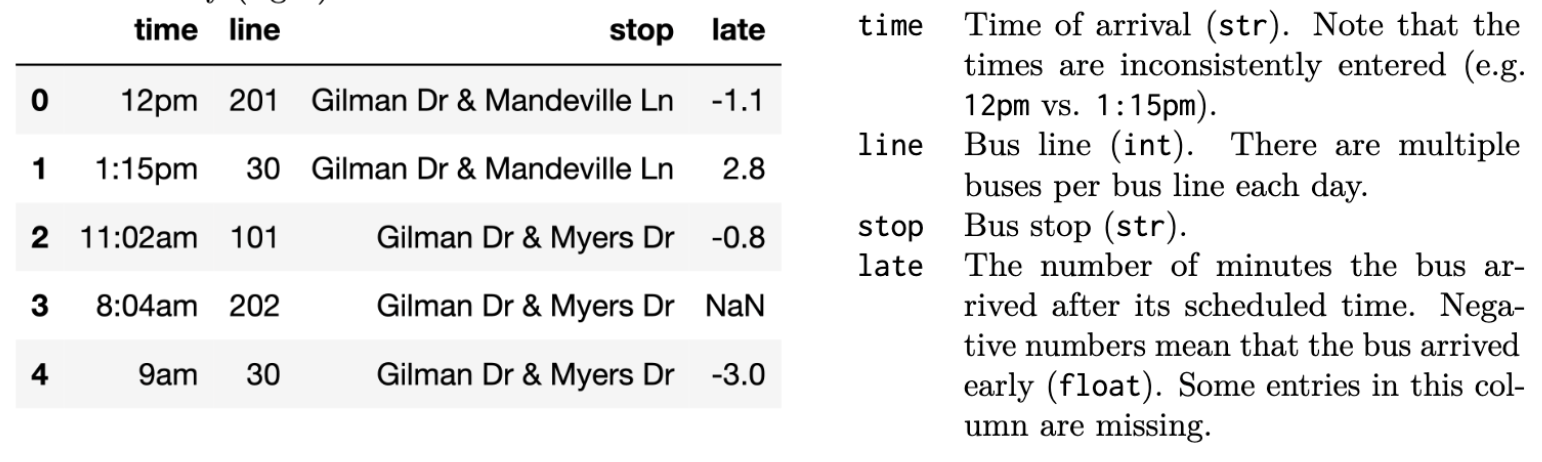
The bus table (left) records bus arrivals over 1 day for all the bust stops within a 2 mile radius of UCSD. The data dictionary
(right) describes each column.
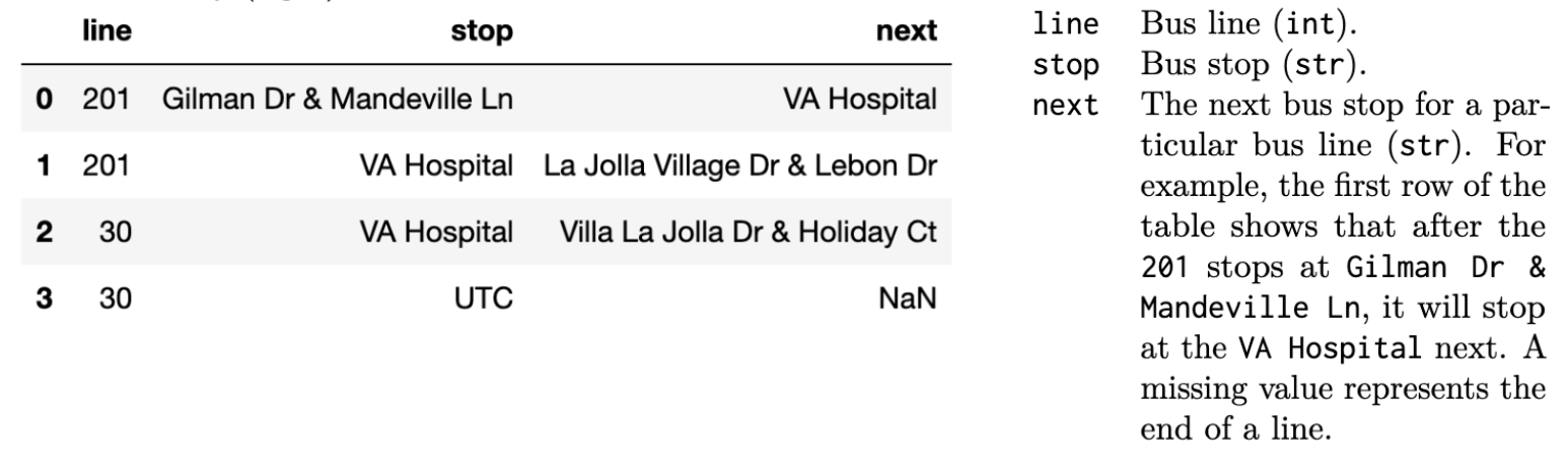
The stop table (left) contains information for al the
bus lines in San Diego (not just the ones near UCSD). The data
dictionary (right) describes each column.
Fill in Python code below so that the last line of each code snippet
evaluates to each desired result, using the bus and
stop DataFrames describe on Page 1 of the Reference Sheet.
You may not use for or while loops in
any answer for this question.
Compute the median minutes late for the 101 bus.
bus.loc[____].median()Answer:
bus.loc[bus['line'] == 101, 'late'].median()
.loc[] will grab the rows of the first argument and
columns of the second argument. In this case, we want all the rows that
belong to bus 101, so we filter by
bus['line'] == 101. We then want to see how late the buses
are, so we grab the 'late' column in the second
argument.
The average score on this problem was 72%.
Compute a copy of bus with only the bus lines that made
at least one stop containing the string 'Myers Ln'.
def f(x):
    return ____
bus.groupby(____).____(f)Answer:
def f(x):
    return x['stop'].str.contains('Myers Ln').sum() > 0
bus.groupby('line').filter(f)
We can start with the bottom groupby method call – since
know we are asked to look per bus line, we will perform
our calculations separately for each bus line ('line').
Then, remember that we’re asked to keep all of the rows for certain bus
lines, meaning that we will need to filter bus lines by
some criteria. To decide which bus lines to keep in our DataFrame, we
must define a function f that takes in a DataFrame
x (which contains all of the rows for one particular bus
line) and returns True if we want to keep that line or
False otherwise. Here, f(x) should return
True if at least one of the values in
x['stop'] contains the string 'Myers Ln'.
x['stop'].str.contains('Myers Ln') will give us a Boolean
Series with True for each 'stop' in
x that contains 'Myers Ln', and
x['stop'].str.contains('Myers Ln').sum() > 0 will check
whether there’s at least one True in that Boolean Series.
This will then return True or False, which
determines if that bus line is kept in our computed DataFrame.
The average score on this problem was 58%.
Compute the number of buses in bus whose next stop is
'UTC'.
x = stop.merge(____, on = ____, how = ____)
x[____].shape[0]Answer:
x = stop.merge(bus, on = ['line', 'stop'], how = 'inner')
x[x['next'] == 'UTC'].shape[0]
OR
x = stop.merge(bus, on = ['line', 'stop'], how = 'right')
x[x['next'] == 'UTC'].shape[0]
OR
x = stop.merge(bus, on = ['line', 'stop'], how = 'left')
x[(x['next'] == 'UTC') & (~x['time'].isna())].shape[0]
OR
x = stop.merge(bus, on = 'line', how = 'left')
x[(x['next'] == 'UTC') & (x['stop_x'] == x['stop_y'])].shape[0]
The top solution is our internal solution, the additional three are
student solutions that we also accepted. First, we merge the
stop DataFrame with the bus DataFrame because
the question specifically wants to know about the number of buses from
the bus DataFrame. We want to merge on both
'line' and 'stop' because we need to find the
number of bus lines that are at a specific stop. We then choose to do an
inner merge, but a right merge has the same effect because the buses in
bus are all in the scope of stop, but
stop has extra bus lines we don’t care about for this
question. Finally, we query our DataFrame x by checking
which ['line', 'stop'] combinations are headed to
'UTC' next by looking at the 'next'
column.
The average score on this problem was 64%.
Computer the number of unique pairs of bus stops that are exactly two
stops away from each other. For example, if you only use the first four
rows of the stop table, then your code should evaluate to
the number 2, since you can go from
'Gilman Dr & Mandeville Ln' to
'La Jolla Village Dr & Lebon Dr' and from
'Gilman Dr & Mandeville Ln' to
'Villa La Jolla Dr & Holiday Ct' in two stops.
Hint: The suffixes = (1, 2) argument to
merge appends a 1 to
column labels in the left table and a 2
to column labels in the right table whenever the merged tables share
column labels.
m = ____.merge(____, left_on = ____, right_on = ____, how = ____, suffixes=(1, 2))
(m[____].drop_duplicates().shape[0])Answer:
m = stop.merge(stop, left_on = 'next', right_on = 'stop', how = 'inner', suffixes=(1, 2))
(m[['stop1', 'next2']].drop_duplicates().shape[0])
We want to look at all stops in San Diego, so we will not be using
the bus DataFrame for this question. Instead, we will merge
stop with itself, but on the left we will merge on the
'next' column, and on the right we will merge on the
'stop' column. This means we get the first stop on the left
DataFrame, the next stop from the left DataFrame matching with the right
DataFrame, and then the next stop from the right DataFrame. That results
in the 'stop' column of the left DataFrame being 2 stops away from the 'next'
column of the right DataFrame. That means all we need to do is use an
inner merge to drop any stops that do not have a match
2 stops away. Since we are now left
with a DataFrame of stops that we want, we just grab the correctly
formatted output by selecting the ['stop1', 'next2']
columns from m, recalling that we use 1 and 2 to
distinguish the columns from the left and right DataFrames.
The average score on this problem was 54%.
Sunan wants to work with the 'time' column in
bus, but the times aren’t consistently formatted. He writes
the following code:
import re

def convert(y1, y2, y3):
    return int(y1), int(y2) if y2 else 0, y3

def parse(x):
    # Fill me in

bus['time'].apply(parse)
Sunan wants the last line of his code to output a Series containing
tuples with parsed information from the 'time' column. Each
tuple should have three elements: the hour, minute, and either
'am' or 'pm' for each time. For example, the
first two values in the 'time' column are
'12pm' and '1:15pm', so the first two tuplies
in the Series should be: (12, 0, 'pm') and
(1, 15, 'pm').
Select all the correct implementations of the
function parse. Assume that each value in the
'time' column starts with aone or two digits for the hour,
followed by an optional colon and an optional two digits for the minute,
followed by either “am” or “pm”.
Hint: Calling .groups() on a regular expression
match object returns the groups of the match as a tuple. For nested
groups, the outermost group is returned first. For example:
>>> re.match(r'(..(...))', 'hello').groups()
('hello', 'llo')
Option A:
def parse(x):
    res = x[:-2].split(':')
    return convert(res[0], res[1] if len(res) == 2 else 0, x[-2:])
Option B:
def parse(x):
    res = re.match(r'(\d+):(\d+)([apm]{2}', x).groups()
    return convert(res[0], res[1], res[2])
Option C:
def parse(x):
    res = re.match(r'(\d+)(:(\d+))?(am|pm)', x).groups()
    return convert(res[0], res[2], res[3])
Option D:
def parse(x):
    res = re.match(r'(.+(.{3})?)(..)', x).groups()
return convert(res[0], res[1], res[2])Answer: Options A and C
'am' /
'pm' with x[:-2]. Then splitting on
':' means that values such as '1:15' become a
list like ['1', '15'], while single numbers such as
'12' become a list like ['12']. We then pass
in the hour value, the minute value or 0 if there is none,
and then the 'am' / 'pm' value by grabbing
just the last two indices of x.x and
return a list of those groups using .groups(). The regex
matches to any number of integers '(\d+)' as the first
group, then a colon ':', another group of any number of
integers '(\d+)', then a final group that matches exactly
twice to characters from “apm”, which can be “am” or “pm” with
'([apm]{2})'. The problem with this solution is that while
it does correctly match to input such as '1:15pm', it would
not match to '12pm' because there is no ':'
character.x and
return a list of those groups using .groups(). The regex
matches to any number of integers '(\d+)' as the first
group, then looks for a colon ':' as the second group, and
matches another group to any number of integers following it with
'(\d+)'. The '?' character makes the previous
matches optional, so if there is no ':' followed by
integers then it will return None for groups 2 and 3 and
still match the rest of the string. Finally, it matches one last group
that is any two characters after the previous groups. This solution
works because the full regex matches the format '1:15pm',
while the '?' checks so if there is no ':' it
can still match something formatted like '12pm'. It also
passes in the group indices 0, 2, and 3 because group 1 will just be
':' or None, so we want to skip it.x and
return a list of those groups using .groups(). The regex
matches any character unlimited times with '.+' as the
first group, then has another group that takes 3 of any character after
the first group from '(.{3})?, and this group is optional
because of the ending '?'. Finally, the last two characters
are the last group '(..)'. This solution does not work
because while the intention is that '.+' grabs the hour and
'(.{3})?' grabs the colon and minutes if present, the
'.+' just grabs everything because the '+'
matches unlimited times. Therefore, '1:15pm' returns the
groups ['1:15', None, 'pm'], which doesn’t work with our
convert function.
The average score on this problem was 81%.
Dylan wants to answer the following questions using hypothesis tests
on the bus DataFrame. For each test, select the
one correct procedure to simulate a single sample under
the null hypothesis, and select the one correct test
statistic for the hypothesis test among the choices given. Assume that
the 'time' column of the bus DataFrame has
already been parsed into timestamps.
Are buses more likely to be late in the morning (before 12 PM) or the afternoon (after 12 PM)? Note: while the problem says there is only one solution, post-exam two options for the test statistic were given credit. Pick one of the two.
Simulation procedure:
np.random.choice([-1, 1], bus.shape[0])
np.random.choice(bus['late'], bus.shape[0], replace = True)
Randomly permute the 'late' column
Test statistic:
Difference in means
Absolute difference in means
Difference in proportions
Absolute difference in proportions
Answer: Simulation procedure: Randomly permute the
'late' column; Test statistic: Difference in means or
difference in proportions
Simulation procedure: We have two samples here: a
sample of 'late' values for buses in the morning and a
sample of 'late' values for buses in the afternoon. The
question is whether the observed difference between these two samples is
statistically significant, making this a permutation test. Note that
Option B is similar, but with replace=True so it is
bootstrapping, not permuting.
Test statistic: Depending on your interpretation of the question, either difference in means or difference in proportions is correct. First, we can’t choose absolute difference as a solution because then we can’t answer when buses will be more likely to be late, as we need the test statistic to be directional to determine which bus category is more likely to be late. If you interpret the question to mean which group of buses has the higher average lateness, then you would want to choose the difference in means; if you interpret the question to mean which group of buses has a higher count of late buses, then you choose difference in proportions.
The average score on this problem was 56%.
Are buses equally likely to be early or late? Note: while the problem says there is only one solution, post-exam two options for the test statistic were given credit. Pick one of the two.
Simulation procedure:
A. np.random.choice([-1, 1], bus.shape[0])
B.
np.random.choice(bus['late'], bus.shape[0], replace = True)
C. Randomly permute the 'late' column
Test statistic:
A. Number of values below 0
B. np.mean
C. np.std
D. TVD
E. K-S statistic
Answer: Simulation procedure:
np.random.choice([-1, 1], bus.shape[0]); Test statistic:
Number of values below 0 or
np.mean
Simulation procedure: The sample we have here is
something like 152 early buses, 125 late buses (these numbers are made
up – in practice, these two numbers need to add to
bus.shape[0]). The question is whether this sample looks
like it was drawn from a population that is 50-50 (an equal number of
early and late buses), which makes this a hypothesis test. In terms of
examples from class, this most closely resembles the very first
hypothesis testing example we looked at – the “coin flipping”
example.
np.random.choice([-1, 1], bus.shape[0]) will return an
array of length bus.shape[0], where each element is equally
likely to be either -1 (late) or 1 (early).
(Note that we could also take -1 to mean early and
1 to mean late – it doesn’t really matter.)
Test statistic: Each time we simulate an arrays of
-1s and 1s, we’d like to compute a statistic
that helps us differentiate between the number of late (-1)
and the number of early (1) simulated buses. The number of
values below 0 will give us the number
of late simulated buses, so we could use that. The mean of the
-1s and 1s will give us a value that is
negative if there were more late buses and positive if there were more
early buses, so we could use that too.
The average score on this problem was 96%.
Is the 'late' column MAR dependent on the
'line' column?
Simulation procedure:
np.random.choice([-1, 1], bus.shape[0])
np.random.choice(bus['late'], bus.shape[0], replace = True)
Randomly permute the 'late' column
Test statistic:
Absolute difference in means
Absolute difference in proportions
TVD
K-S statistic
Answer: Simulation procedure: Randomly permute the
'late' column; Test statistic: TVD
Simulation procedure: To determine if
'late' is missing at random dependent on the
'line' column, we conduct a permutation test and compare
(1) the distribution of the 'line' column when the
'late' column is missing to (2) the distribution of the
'line' column when the 'late' column is not
missing to see whether they’re significantly different. If the
distributions are indeed significantly different, then it is likely that
the 'late' column is MAR dependent on 'line'.
Test statistic: Since we are comparing the
distributions of categorical data ('line' is
categorical) for our permutation test, Total Variation Distance is the
best test statistic to use.
The average score on this problem was 57%.
Is the 'late' column MAR dependent on the
'time' column?
Simulation procedure:
A. np.random.choice([-1, 1], bus.shape[0])
B.
np.random.choice(bus['late'], bus.shape[0], replace = True)
C. Randomly permute the 'late' column
Test statistic:
A. Absolute difference in proportions
B. TVD
C. K-S statistic
Answer: Simulation procedure: Randomly permute the
'late' column; Test statistic: K-S statistic
Simulation procedure: Like in the previous part, to
determine if 'late' is missing at random dependent on the
'time' column, we conduct a permutation test and compare
(1) the distribution of the 'time' column when the
'late' column is missing to (2) the distribution of the
'time' column when the 'late' column is not
missing to see whether they’re significantly different.
Test statistic: Since we are comparing the
distributions of numerical data ('time' is
numerical) for our permutation test, K-S statistic is the best test
statistic to use of the options provided.
Answer the following questions about missingness mechanisms. For each question, choose either not missing at random (NMAR), missing at random (MAR), missing completely at random (MCAR), or missing by design (MD).
What is the missingness mechanism for the 'next' column
in the stop DataFrame?
Answer: Missing by design (MD)
When there are missing values for the 'next' column, it
means there is no next stop and the line has reached the end of its
route. This could have been designed differently to have an empty
string, a string saying "end", etc. Therefore, the missing
values are intentionally marked as missing by design.
The average score on this problem was 68%.
Suppose that the missing values in the 'late' column
from the bus DataFrame are missing because Sam got
suspicious of negative values and deleted a few of them. What is the
missingness mechanism for the values in the 'late'
column?
Answer: Not missing at random (NMAR)
Since Sam deleted 'late' values that were negative, the
missingness of 'late' values depends on the values
themselves, making the missingness mechanism not missing at random.
The average score on this problem was 86%.
Suppose that the missing values in the 'late' column
from the bus DataFrame are missing because Tiffany made an
update to the GPS system at 8 AM and the system was down for 15 minutes afterwards. What is the
missingness mechanism for the values in the late
column?
Answer: Missing at random (MAR)
Since Tiffany updated the system at 8 AM, the missing values in
'late' are dependent on the 'time' column.
Therefore, 'late' values are missing at random.
The average score on this problem was 68%.
Giorgia defines the following variables:
a = bus['late'].mean()
b = bus['late'].std()
She applies the imputation methods below to the 'late'
column, then recalculates a and b. For each
imputation method, choose whether the new values of a and
b will be lower (-),
higher (+), exactly the same (=), or approximately the same (\approx) as the original values of
a and b.
Mean imputation
Answer: a’s new value will be exactly
the same as before (=);
b’s new value will be lower than before (-)
By replacing all of the missing values in the 'late'
column with the observed mean, the mean value won’t change. However, the
squared distances of values to the mean, on average, will decrease,
because the imputed dataset will be less spread out, so the standard
deviation will decrease.
Probabilistic imputation
Answer: a’s new value will be
approximately the same as before (\approx); b’s new value will be
approximately the same as before (\approx)
Now, to fill in missing values, we’re sampling at random from the originally observed set of values. The shape of the imputed distribution will be similar to the shape of the original distribution, so its mean and standard deviation will be similar to that of the original distribution (though not necessarily exactly equal).
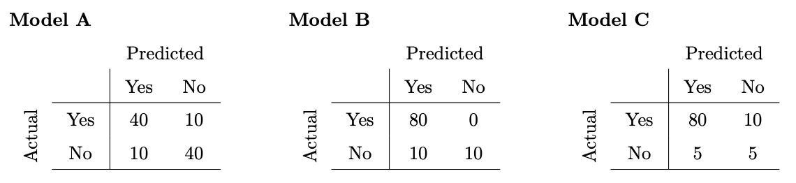
Consider three classifiers with the following confusion matrices:
Which model has the highest accuracy?
Model A
Model B
Model C
Answer: Model B
Accuracy is defined as \frac{\text{number\;of\;correct\;predictions}}{\text{number\;of\;total\;predictions}}, so we sum the (Yes, Yes) and (No, No) cells to get the number of correct predictions and divide that by the sum of all cells as the number of total predictions. We see that Model B has the highest accuracy of 0.9 with that formula. (Note that for simplicity, the confusion matrices are such that the sum of all values is 100 in all three cases.)
The average score on this problem was 98%.
Which model has the highest precision?
Model A
Model B
Model C
Answer: Model C
Precision is defined as \frac{\text{number of correctly predicted yes values}}{\text{total number of yes predictions}}, so the number of correctly predicted yes values is the (Yes, Yes) cell, while the total number of yes predictions is the sum of the Yes column. We see that Model C has the highest precision, \frac{80}{85}, with that formula.
The average score on this problem was 86%.
Which model has the highest recall?
Model A
Model B
Model C
Answer: Model B
Recall is defined as \frac{\text{number of correctly predicted yes values}}{\text{total number of values actually yes}}, so the number of correctly predicted yes values is the (Yes, Yes) cell, while the total number of values that are actually yes is the sum of the Yes row. We see that Model B has the highest recall, 1, with that formula.
The average score on this problem was 83%.
Alan set up a web page for his DSC 80 note swith the following HTML:
<html>
    <body>
        <div id = "hero">DSC 80 NOTES</div>
        <div class="notes">
            <div class="notes">
                <p>Lecture 1: 5/5 stars!</p>
            </div>
            <div class="lecture notes">
                <p>Lecture 2: 6/5 stars!!</p>
            </div>
        </div>
        <div class="lecture">
            <p>Lecture 3: 10/5 stars!!!!</p>
        </div>
    </body>
</html>
Assume that the web page is parsed into a BeautifulSoup objected
named soup. Fill in each of the expressions below to
evaluate to the desired string. Pay careful attention to the indexes
after each call to find_all!
Desired string: "Lecture 1: 5/5 stars!"
soup.find_all(____)[0].textAnswer: soup.find_all('p')[0].text
"Lecture 1: 5/5 stars!" is surrounded by
<p> tags, and find_all will get every
instance of these tags as a list. Since
"Lecture 1: 5/5 stars!" is the first instance, we can get
it from its index in the list, [0]. Then we grab just the
text using .text.
The average score on this problem was 87%.
Desired string: "Lecture 2: 6/5 stars!!"
soup.find_all(____)[3].textAnswer:
soup.find_all('div')[3].text
"Lecture 2: 6/5 stars!!" appears as the text surrounded
by the fourth <div> tag, and since we are grabbing
index [3] we need to find_all('div'). Then
.text grabs the text portion.
The average score on this problem was 82%.
Desired string: "Lecture 3: 10/5 stars!!!!"
soup.find_all(____)[1].textAnswer:
soup.find_all('div', class_='lecture')[1].text
We need to return a list with
"Lecture 3: 10/5 stars!!!!" as the second index since we
access it with [1]. We see that we have two instances of
'lecture' attributes in div tags: one with
class="lecture notes" and class="lecture".
Note that class="lecture notes" actually means that the tag
has two class attributes, one of "lecture" and
one of "notes". The class_='lecture' optional
argument in find_all will find all tags that have a
'lecture' attribute, meaning that it’ll find both the
class="lecture notes" tag and the
class="lecture" tag. So,
soup.find_all('div', class_='lecture') will find the two
aforementioned <div>s, [1] will find the
second one (which is the one we want), and .text will find
"Lecture 3: 10/5 stars!!!!".
The average score on this problem was 74%.
Consider the following corpus:
| Document number | Content |
|---|---|
| 1 | yesterday rainy today sunny |
| 2 | yesterday sunny today sunny |
| 3 | today rainy yesterday today |
| 4 | yesterday yesterday today today |
Using a bag-of-words representation, which two documents have the largest dot product? Show your work, then write your final answer in the blanks below.
Documents ____ and ____
Answer: Documents 3 and 4
The bag-of-words representation for the documents is:
| Document number | yesterday | rainy | today | sunny |
|---|---|---|---|---|
| 1 | 1 | 1 | 1 | 1 |
| 2 | 1 | 0 | 1 | 2 |
| 3 | 1 | 1 | 2 | 0 |
| 4 | 2 | 0 | 2 | 0 |
The dot product between documents 3 and 4 is 6, which is the highest among all pairs of documents.
The average score on this problem was 84%.
Using a bag-of-words representation, what is the cosine similarity between documents 2 and 3? Show your work below, then write your final answer in the blank below.
Answer: \frac{1}{2}
The dot product between documents 2 and 3 is: 1 + 0 + 2 + 0 = 3 The magnitude of document 2 is equal to document 3 and is: \sqrt{1^2 + 0 ^2 + 1^2 + 2^2} = \sqrt{6} So, the cosine similarity is \frac{3}{\sqrt{6}\times\sqrt{6}} = \frac{1}{2}
The average score on this problem was 70%.
Which words have a TF-IDF score 0 for all four documents? Assume that we use base-2 logarithms. Select all the words that apply.
yesterday
rainy
today
sunny
Answer: yesterday and today
Remember,
\text{tf-idf}(t, d) = \text{tf}(t, d) \cdot \text{idf}(t)
where \text{tf}(d, t), the term frequency of term t in document d, is the proportion of terms in d that are equal to t, and \text{idf}(t) = \log \left( \frac{\text{number of documents}}{\text{number of documents containing $t$}} \right).
In order for \text{tf-idf}(t, d) to be 0, either t must not be in document d (meaning \text{tf}(t, d) = 0), or t is in every document (meaning \text{idf}(t) = \log(\frac{n}{n}) = \log(1) = 0). In this case, we’re looking for words that have a \text{tf-idf} of 0 across all documents, which means we’re looking for words that have a \text{idf}(t) of 0, meaning they’re in every document. The words that are in every document are yesterday and today.
The average score on this problem was 94%.
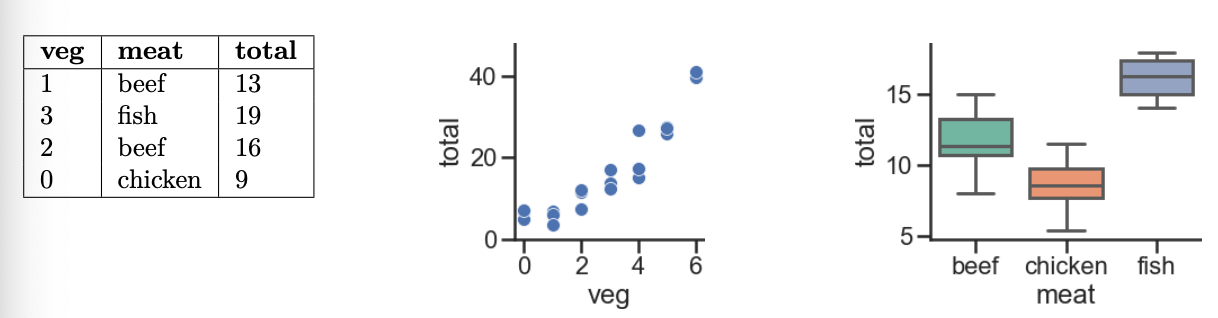
Every week, Lauren goes to her local grocery store and buys a varying amount of vegetable but always buys exactly one pound of meat (either beef, fish, or chicken). We use a linear regression model to predict her total grocery bill. We’ve collected a dataset containing the pounds of vegetables bought, the type of meat bought, and the total bill. Below we display the first few rows of the dataset and two plots generated using the entire training set.
Suppose we fit the following linear regression models to predict
'total' using the squared loss function. Based on the data
and visualizations shown above, for each of the following models H(x), determine whether each fitted
model coefficient w^* is
positive (+), negative (-), or exactly 0. The notation \text{meat=beef} refers to the one-hot
encoded 'meat' column with value 1 if the original value in the
'meat' column was 'beef' and 0 otherwise. Likewise, \text{meat=chicken} and \text{meat=fish} are the one-hot encoded
'meat' columns for 'chicken' and
'fish', respectively.
For example, in part (iv), you’ll need to provide three answers: one for w_0^* (either positive, negative, or 0), one for w_1^* (either positive, negative, or 0), and one for w_2^* (either positive, negative, or 0).
Model i. H(x) = w_0
Answer: w_0^* must
be positive
If H(x) = w_0, then w_0^* will be the mean 'total'
value in our dataset, and since all of our observed 'total'
values are positive, their mean – and hence, w_0^* – must also be positive.
Model ii. H(x) = w_0 + w_1 \cdot
\text{veg}
Answer: w_0^* must be positive; w_1^* must be positive
Of the three graphs provided, the middle one shows the relationship
between 'total' and 'veg'. We see that if we
were to draw a line of best fit, the y-intercept (w_0^*) would be positive, and so would the
slope (w_1^*).
Model iii. H(x) = w_0 + w_1 \cdot
\text{(meat=chicken)}
Answer: w_0^* must be positive; w_1^* must be negative
Here’s the key to solving this part (and the following few): the
input x has a 'meat' of
'chicken', H(x) = w_0 +
w_1. If the input x has a
'meat' of something other than 'chicken', then
H(x) = w_0. So:
'total' prediction that makes sense for non-chicken inputs,
and'total' prediction for chickens.For all three 'meat' categories, the average observed
'total' value is positive, so it would make sense that for
non-chickens, the constant prediction w_0^* is positive. Based on the third graph,
it seems that 'chicken's tend to have a lower
'total' value on average than the other two categories, so
if the input x is a
'chicken' (that is, if \text{meat=chicken} = 1), then the constant
'total' prediction should be less than the constant
'total' prediction for other 'meat's. Since we
want w_0^* + w_1^* to be less than w_0^*, w_1^*
must then be negative.
Model iv. H(x) = w_0 + w_1 \cdot
\text{(meat=beef)} + w_2 \cdot \text{(meat=chicken)}
Answer: w_0^* must
be positive; w_1^* must be negative;
w_2^* must be negative
H(x) makes one of three predictions:
'meat'
value of 'chicken', then it predicts w_0 + w_2.'meat'
value of 'beef', then it predicts w_0 + w_1.'meat'
value of 'fish', then it predicts w_0.Think of w_1^* and w_2^* – the optimal w_1 and w_2
– as being adjustments to the mean 'total' amount for
'fish'. Per the third graph, 'fish' have the
highest mean 'total' amount of the three
'meat' types, so w_0^*
should be positive while w_1^* and
w_2^* should be negative.
Model v. H(x) = w_0 + w_1 \cdot
\text{(meat=beef)} + w_2 \cdot \text{(meat=chicken)} + w_3 \cdot
\text{(meat=fish)}
Answer: Not
enough information for any of the four coefficients!
Like in the previous part, H(x) makes one of three predictions:
'meat'
value of 'chicken', then it predicts w_0 + w_2.'meat'
value of 'beef', then it predicts w_0 + w_1.'meat'
value of 'fish', then it predicts w_0 + w_3.Since the mean minimizes mean squared error for the constant model,
we’d expect w_0^* + w_2^* to be the
mean 'total' for 'chicken', w_0^* + w_1^* to be the mean
'total' for 'beef', and w_0^* + w_3^* to be the mean total for
'fish'. The issue is that there are infinitely many
combinations of w_0^*, w_1^*, w_2^*,
w_3^* that allow this to happen!
Pretend, for example, that:
'total' for 'chicken is 8.'total' for 'beef' is 12.'total' for 'fish' is 15.Then, w_0^* = -10, w_1^* = 22, w_2^* = 18, w_3^* = 25 and w_0^* = 20, w_1^* = -8, w_2^* = -12, w_3^* = -5 work, but the signs of the coefficients are inconsistent. As such, it’s impossible to tell!
Suppose we fit the model H(x) = w_0 + w_1 \cdot \text{veg} + w_2 \cdot \text{(meat=beef)} + w_3 \cdot \text{(meat=fish)}. After fitting, we find that \vec{w^*}=[-3, 5, 8, 12]
What is the prediction of this model on the first point in our dataset?
-3
2
5
10
13
22
25
Answer: 10
Plugging in our weights \vec{w}^* to the model H(x) and filling in data from the row
| veg | meat | total |
|---|---|---|
| 1 | beef | 13 |
gives us -3 + 5(1) + 8(1) + 12(0) = 10.
The average score on this problem was 93%.
Following the same model H(x) and weights from the previous problem, what is the loss of this model on the second point in our dataset, using squared error loss?
0
1
5
6
8
24
25
169
Answer: 25
The squared loss for a single point is (\text{actual} - \text{predicted})^2. Here,
our actual 'total' value is 19, and our predicted value
'total' value is -3 + 5(3) + 8(0)
+ 12(1) = -3 + 15 + 12 = 24, so the squared loss is (19 - 24)^2 = (-5)^2 = 25.
The average score on this problem was 84%.
Determine how each change below affects model bias and variance compared to the model H(x) described at the top of this page. For each change (i., ii., iii., iv.), choose all of the following that apply: increase bias, decrease bias, increase variance, decrease variance.
'veg' feature.Suppose we predict 'total' from 'veg' using
8 models with different degree
polynomial features (degrees 0 through
7). Which of the following plots
display the training and validation errors of these models? Assume that
we plot the degree of the polynomial features on the x-axis, mean
squared error loss on the y-axis, and the plots share y-axes limits.
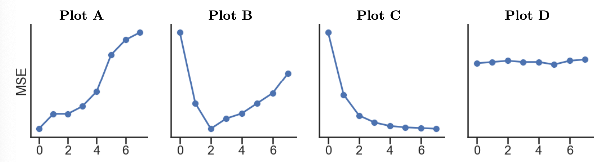
Training Error:
A
B
C
D
Validation Error:
A
B
C
D
Answer: Training error: C; Validation Error: B
Training Error: As we increase the complexity of our model, it will gain the ability to memorize the patterns in our training set to a greater degree, meaning that its performance will get better and better (here, meaning that its MSE will get lower and lower).
Validation Error: As we increase the complexity of
our model, there will be a point at which it becomes “too complex” and
overfits to insignificant patterns in the training set. The second graph
from the start of Problem 9 tells us that the relationship between
'total' and 'veg' is roughly quadratic,
meaning it’s best modeled using degree 2 polynomial features. Using a degree greater
than 2 will lead to overfitting and,
therefore, worse validation set performance. Plot B shows MSE decrease
until d = 2 and increase afterwards,
which matches the previous explanation.
The average score on this problem was 88%.
Suppose we fit decision trees of varying depths to predict
'y' using 'x1' and 'x2'. The
entire training set is shown in the table below.
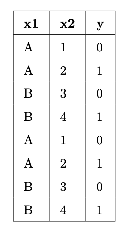
For each option below, select one answer from the list:
0
0.5
1
2
'y' value) and p_C
represents the proportion of points in that node belonging to class
C. In our training set, there are two
classes, 0 and 1, each contaning a proportion p_0 = p_1 = \frac{1}{2} of the values. So,
the entropy of a node that contains our entire training set is -\frac{1}{2} \log_2 \left( \frac{1}{2} \right) -
\frac{1}{2} \log_2 \left( \frac{1}{2} \right) = - \log_2 \left(
\frac{1}{2} \right) = \log_2 2 = 1'y' value). In such a node,
the one class C has a proportion p_C = 1 of the points, and the corresponding
entropy is -p_C \log_2 p_C = -1 \log_2 1 = - 1
\cdot 0 = 0. Here, we can construct a pure node by asking a
question like x_2 \leq 1. There are two
points with x_2 \leq 1; they have y values of [0,
0]. There are six points with x_2 >
1; they have y values of [0, 0, 1, 1, 1, 1]. The entropy of the [0, 0] node is 0.
The average score on this problem was 52%.
Suppose we write the following code:
hyperparameters = {
    'n_estimators': [10, 100, 1000], # number of trees per forest
    'max_depth': [None, 100, 10]     # max depth of each tree
}
grids = GridSearchCV(
    RandomForestClassifier(), param_grid=hyperparameters,
    cv=3, # 3-fold cross-validation
)
grids.fit(X_train, y_train)
Answer the following questions with a single number.
X_train
used to train a decision tree?n_estimators and 3 values for
max_depth. So, the total number of random forests fit is
3 \cdot 3 \cdot 3 = 27.n_estimators
hyperparameter. For instance, a random forest that has
n_estimators=10 is made up of 10 decision trees. The
question is, then, how many times do we fit a random forest with 10
decision trees (10 because it’s the first value in
n_estimators)? The answer is 9, which is the value of k (3) multiplied by the number of values for
max_depth that are being tested – remember, k times, we fit a random forest with each
combination of n_estimators and max_depth. So,
9 times, a random forest with 10 decision trees is fit – but also, 9
times, a random forest with 100 decision trees is fit, and 9 times, a
random forest with 1000 decision trees is fit. So, how many total
decision trees are fit? 9 \cdot (10 + 100 +
1000) = 9 \cdot 1110 = 9990X_train belongs to just one
of these three folds, meaning for every combination of hyperparameters
it’s used for training twice (and validation once). For
n_estimators=10, X_train is used for training
a random forest 3 \cdot 2 times, which
means it’s used for training a decision tree 10 \cdot 3 \cdot 2 times. Following this
logic for n_estimators=100 and
n_estimators=1000 and summing the results gives us (10 + 100 + 1000) (3 \cdot 2) = 1110 \cdot 6 =
6660 So, the first point in X_train is used to train
a decision tree 6660 times.
The average score on this problem was 41%.